The NavimetriX interface has been designed to be clear, intuitive, and quick to use, whether on a computer, tablet, or smartphone. Here is a complete description, section by section:
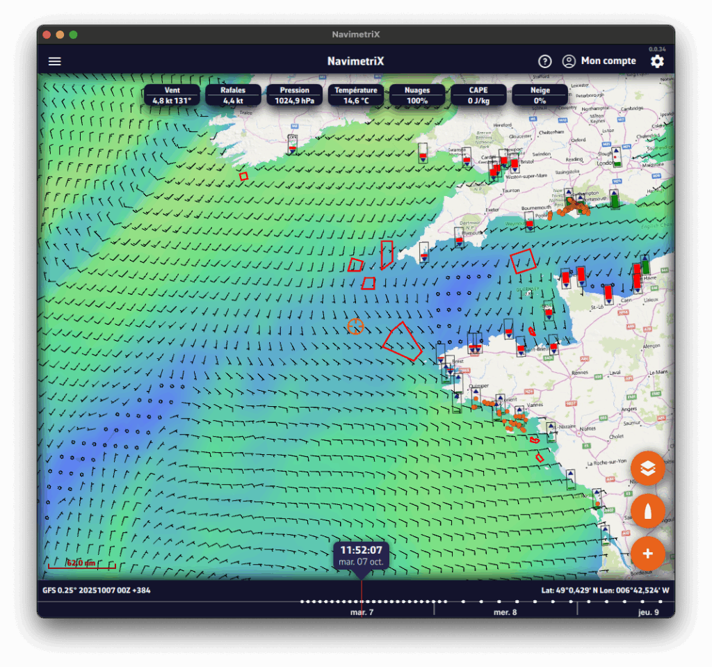
☰ Hamburger menu: provides access to the application’s main lists:
In order for NavimetriX to be synchronised across two or more devices, you must:
Most settings are synchronised, with a few exceptions, namely:


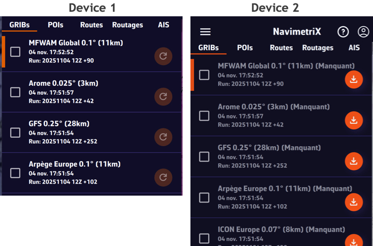
Downloaded GRIB files appear in the GRIB list on all devices. When a GRIB is downloaded or updated on a device, it is followed by a dimmed refresh icon. If a new run is available for that GRIB, this icon is activated.

On other device(s), the list of downloaded GRIBs is displayed but followed by an activated download icon. The contents of the GRIBs must then be downloaded manually.
The Geogarage account is synchronised across all devices.
Geogarage charting is not synchronised: charts must be downloaded to each device.
You will find a short tutorial on the basic functions of NavimetriX by following Get Started.
Before writing to us, please check the FAQs — you’ll probably find the answer to your question 😉.
There’s no need to browse through all the FAQs one by one: you can search within the FAQs, so don’t hesitate to use the search bar!
📘 This glossary brings together the main terms used in the Navimetrix application and its FAQs. It helps users better understand concepts related to navigation, routing, and marine weather.
The actual direction of the boat’s movement over the seabed, expressed in degrees relative to true north. It differs from the compass heading when there is drift caused by wind or current.
The boat’s actual speed relative to the ground (not the water). Calculated by GPS, it includes the effect of currents.
The direction in which the boat’s bow is pointing, measured relative to true or magnetic north.
The angle between the boat’s axis and the true wind direction. It is calculated from the apparent wind and the boat’s speed.
The wind speed derived from the apparent wind and the boat’s speed. It represents the actual wind strength on the sea surface.
The wind angle felt on board, influenced by the boat’s motion. Measured relative to the boat’s centerline.
The wind speed felt on the boat, resulting from the combination of the true wind and the boat’s speed.
The useful component of the boat’s speed, indicating the effective progress toward the destination or upwind.
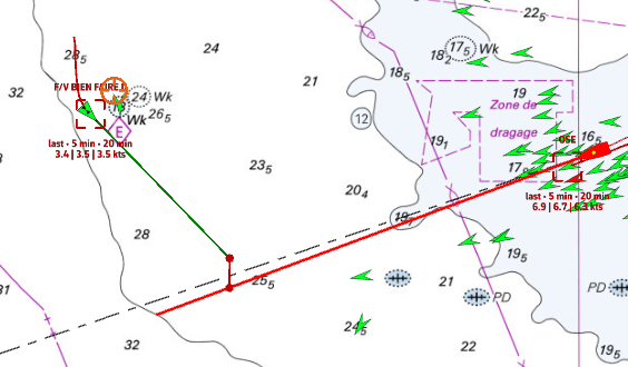
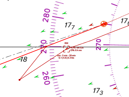
The point at which two vessels will be at their minimum distance from each other, based on their current courses and speeds.
The time remaining before reaching the CPA, used for collision avoidance and AIS alarms.
The angle between north and the direction of an observed object from the boat. Used to determine the relative position of a target or coastline.
The water depth below the keel, measured by an echo sounder. A key parameter for safe navigation.
A geographic point used to define a route or a key position. In Navimetrix, POIs represent these waypoints.
A standard file format containing numerical weather forecasts (wind, waves, pressure, temperature, etc.).
A curve connecting all possible boat positions at a given time according to the predicted weather conditions.
The calculation of an optimal route considering wind, waves, currents, and the boat’s performance.
A performance curve showing the boat’s speed as a function of wind angle and wind strength. It forms the basis for the routing engine.
The predicted time of arrival at the destination, calculated from the remaining distance and the average speed.
A description of the waves and swell (height, direction, period). Used to assess routing comfort and safety.
A regular train of waves formed by distant winds. It differs from the wind sea, which is generated locally.
The average height of the highest one-third of waves, the main indicator of overall sea conditions.
Water movements caused by tides or ocean circulation. They affect the boat’s speed and trajectory.
Variation in sea level caused by the gravitational attraction of the Moon and the Sun. It influences depth and coastal currents.
These operating system versions are prerequisites for running NavimetriX, as they define compatibility with our development framework.
However, they do not guarantee that the application will be fully compatible with your device. Other factors such as insufficient RAM or a low-performance graphics processor may also affect performance and compatibility.
⚠️ If you receive a warning from your antivirus, it is most likely a false positive.
You can check on VirusTotal that our .exe file is clean and recognized as safe by major antivirus programs.
Resolving an issue on a Windows PC can be complex, given the wide variety of possible configurations. Here are some basic steps to check:
If these steps do not solve the problem, your PC may not be compatible due to insufficient RAM or a graphics card that does not meet the app’s requirements.
To uninstall the application:
The application will be uninstalled, and all folders where it stores data as well as its registry keys will be removed.
You can also use the CleanMyMac application.
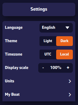
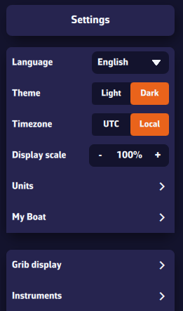
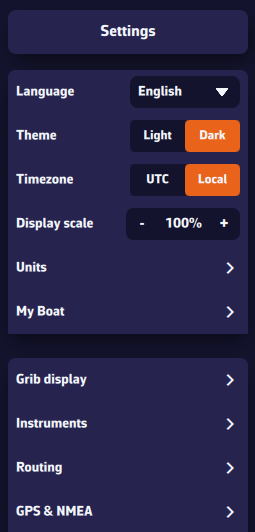
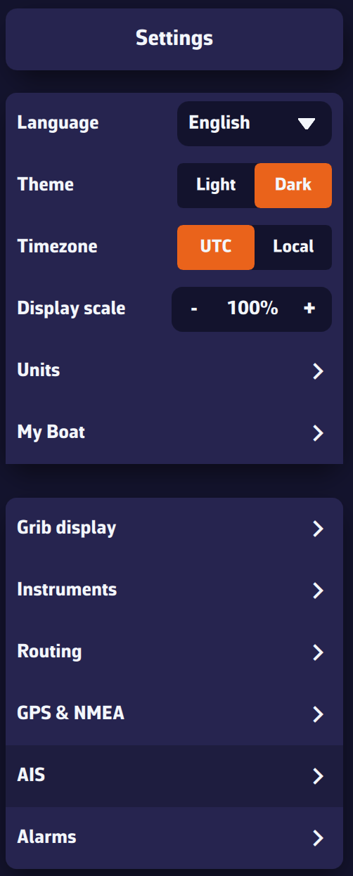
In the Settings panel, the first section covers the basic configuration options:
With a Premium subscription, you’ll enjoy the full potential of the application.
In addition to all the features of the free version:
You’ll benefit from a 7-day free trial period, so don’t hesitate to give it a try — we’re confident you’ll be convinced.
The Premium subscription is annual and renews automatically.
The price depends on the region where you subscribe.
For example, it is:
Please note that the subscription does not include nautical charts. To navigate with marine charts, you need to have a subscription on the Geogarage platform.
At the moment, you cannot subscribe directly from a Windows PC. To get a subscription, please use your phone (or tablet) via the App Store for iOS or macOS, or the Play Store for Android.
This subscription will then be valid on all your devices, including your PC.
When renewing a subscription or at the end of the trial period, in order to update our database with the information provided by the App Store, you must launch the application on the device that took out the subscription.
Important: On your PC or any device where you did not take your subscription, make sure to login to your NavimetriX account to see your subscription
Cancellation is done through your Apple account.
To turn off an automatically renewing subscription on an Apple device (iOS/iPadOS):
Settings > Your Account > Subscriptions > Select the subscription > Cancel Subscription
To cancel a subscription on a Mac, follow this link.
Note: Do not cancel before the end of the 7-day free trial if you wish to keep Premium access. However, if you do not want to subscribe, you must cancel before the end of the 7th day to avoid being charged.
Cancellation is done through your Play Store account.
To turn off an automatically renewing subscription on an Android device:
Follow the instructions on this page.
Note: Do not cancel before the end of the 7-day free trial if you wish to keep Premium access. However, if you do not want to subscribe, you must cancel before the end of the 7th day to avoid being charged.
The NavimetriX interface has been designed to be clear, intuitive, and quick to use, whether on a computer, tablet, or smartphone. Here is a complete description, section by section:
☰ Hamburger menu: provides access to the application’s main lists:
In order for NavimetriX to be synchronised across two or more devices, you must:
Most settings are synchronised, with a few exceptions, namely:
Downloaded GRIB files appear in the GRIB list on all devices. When a GRIB is downloaded or updated on a device, it is followed by a dimmed refresh icon. If a new run is available for that GRIB, this icon is activated.
On other device(s), the list of downloaded GRIBs is displayed but followed by an activated download icon. The contents of the GRIBs must then be downloaded manually.
The Geogarage account is synchronised across all devices.
Geogarage charting is not synchronised: charts must be downloaded to each device.
In the Settings panel, the first section covers the basic configuration options:
Some settings are essential — both for safety and for the proper functioning of the application.
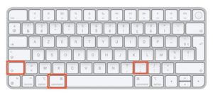
You and your crew members must be able to access the navigation app instantly, whatever the situation. At sea, a code is useless — even dangerous if you are unable to handle navigation yourself: your crew must be able to take over quickly.
Unexpected sleep mode during a critical navigation moment (e.g., nighttime landfall in the rain in an unknown area) can be dangerous if you cannot instantly relaunch the app (e.g., wet fingers or touchscreen not responding). You should manually activate or deactivate your device depending on the situation.
In addition, sleep mode interrupts track recording.
This prevents wasting time when entering text in the app, such as route names, POIs, etc.
Regarding onboard computers, PC or Mac, the same recommendations apply. Adjust the settings according to the operating system and version used.
This setting allows you to enlarge or reduce the size of all elements displayed on the map (up to 140%, for example). Very useful on board if you want to use the app without wearing your glasses.
Note that the menu font size remains unchanged.
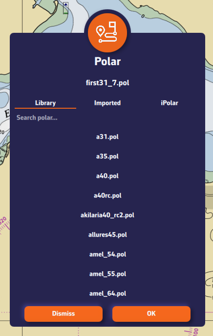
Your boat’s polar determines all routing calculations. It represents your boat’s performance depending on wind speed and angle.
The application supports files in the .pol format (also used by Weather4D, SailGrib, Adrena, and others).
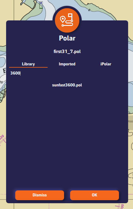
To choose your boat’s polar from the library:
Most of these polars come from naval architects or ORC certificates.
To find your polar, you can:
Once you’ve found your polar, select it and it will be confirmed.
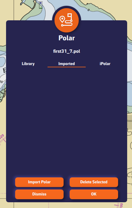
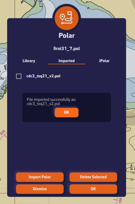
Comment importer une polaire?
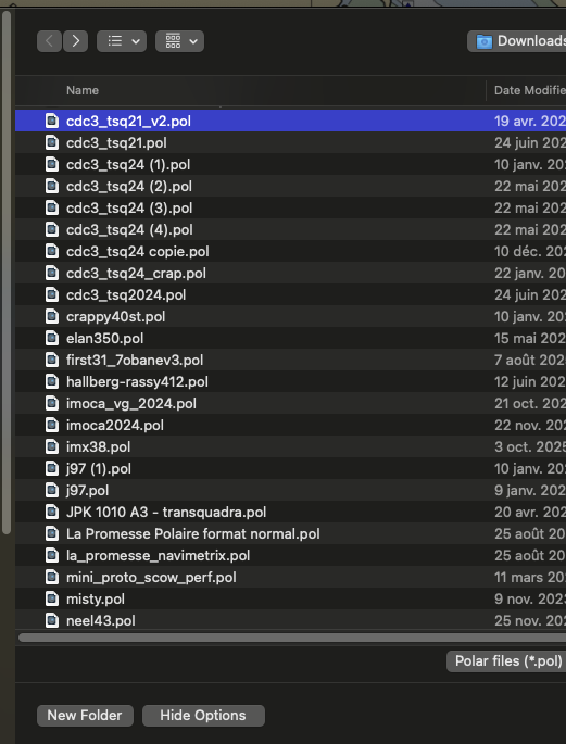
The application can import polars in the .pol format.
To import your own polar:
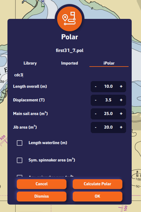
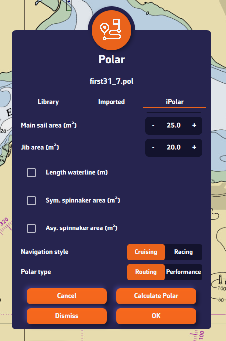
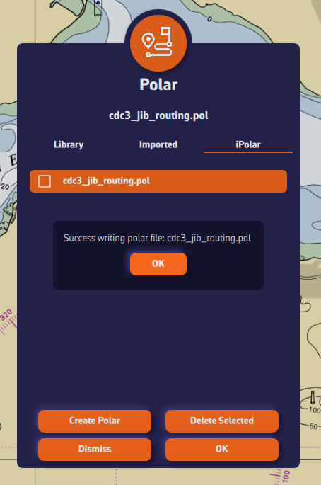
iPolar lets you create a polar in one minute based on your boat’s characteristics:
Note: The iPolar method was developed by KND, experts who work with the America’s Cup, TP52s, and IMOCAs — the best in their field!

Some polars are formatted as .CSV (Comma Separated Value) files, where the field separator is a comma or semicolon. This format is not supported in NavimetriX, unlike the .POL format where fields are separated by tabs — a format widely used in navigation applications. Therefore, you need to convert your .CSV file to .POL.
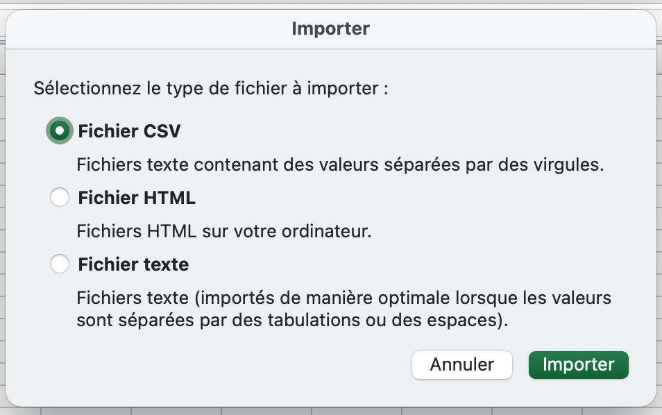
Open a new Excel sheet and select the menu: File > Import.
Choose “CSV File” and then select your polar file from the Finder.
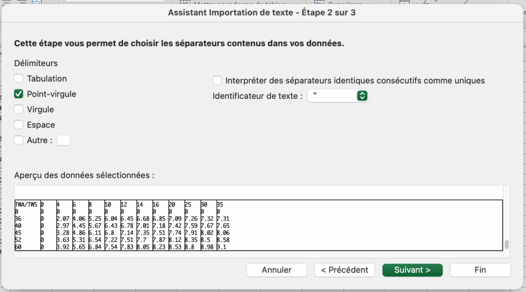
Check the box Delimiters = “Semicolon”, then insert the data into the existing sheet.
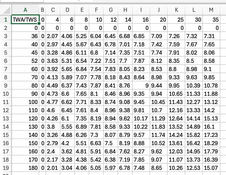
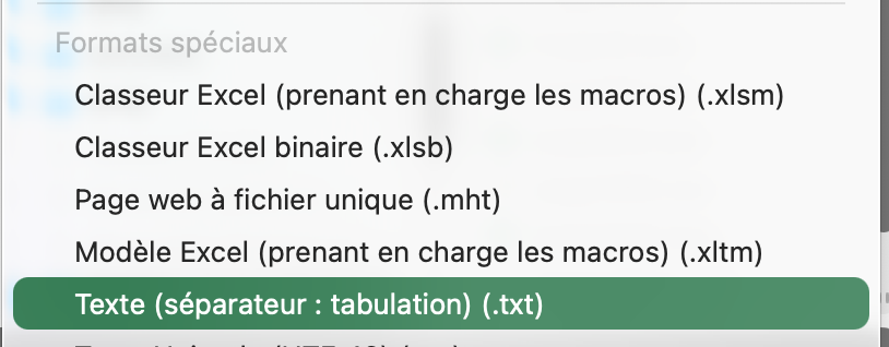
Then save the file in “Text (Tab delimited)” format, which will create a .TXT text file.
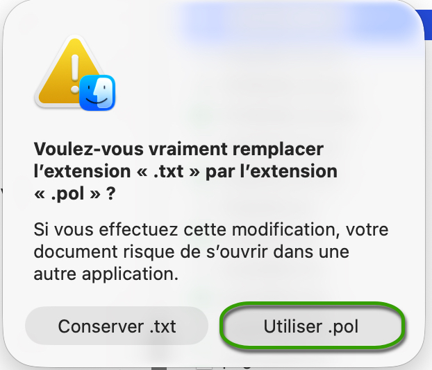
Finally, rename the file by replacing the .TXT extension with .POL:
Your polar file is now ready to be imported.
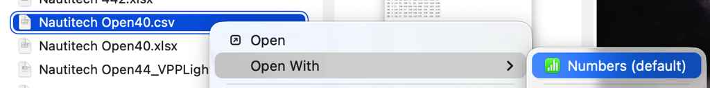
Open the .CSV file with Numbers:
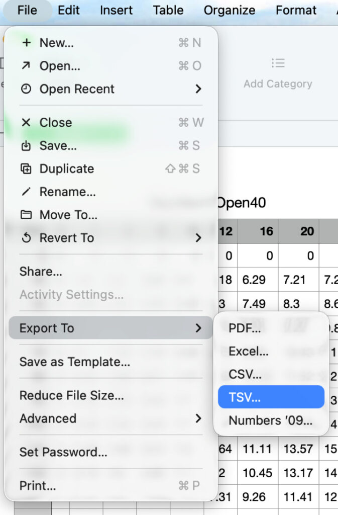
Export the file to TSV:
Replace the file .TSV extension to .POL, that’s all.
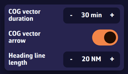
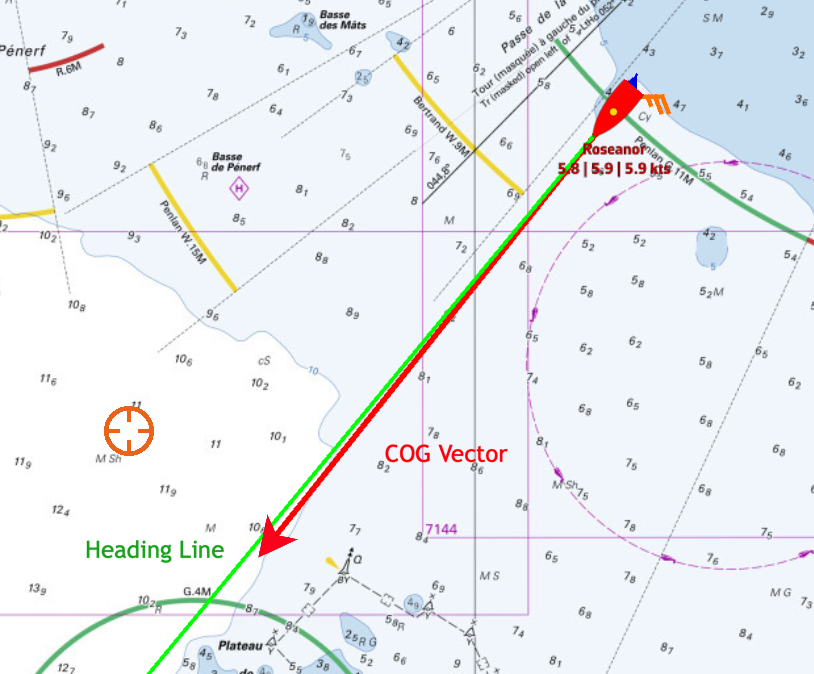
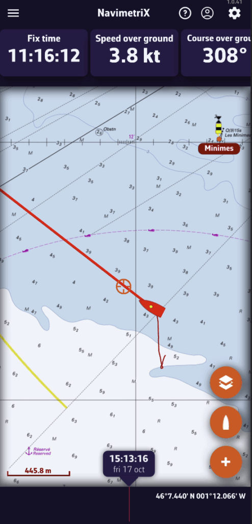
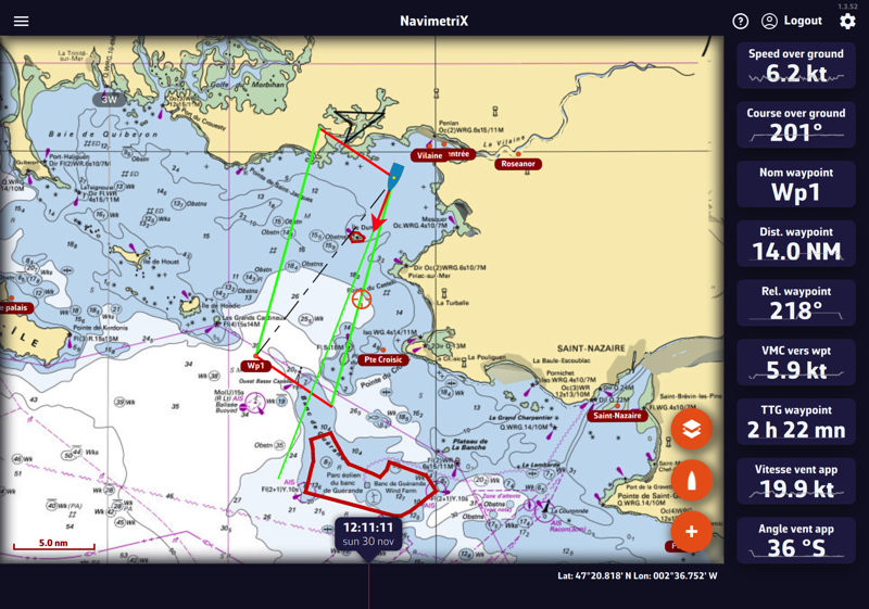
On the chart, the course vector on the ground COG is represented by a red arrow. The magnetic heading line is represented by a green line. Both are variable in length.
Open the app settings by tapping on the ⚙︎ icon, then select the My Boat section.
Open the app settings ⚙︎ and select ‘My boat’. The track settings are at the bottom of the list.
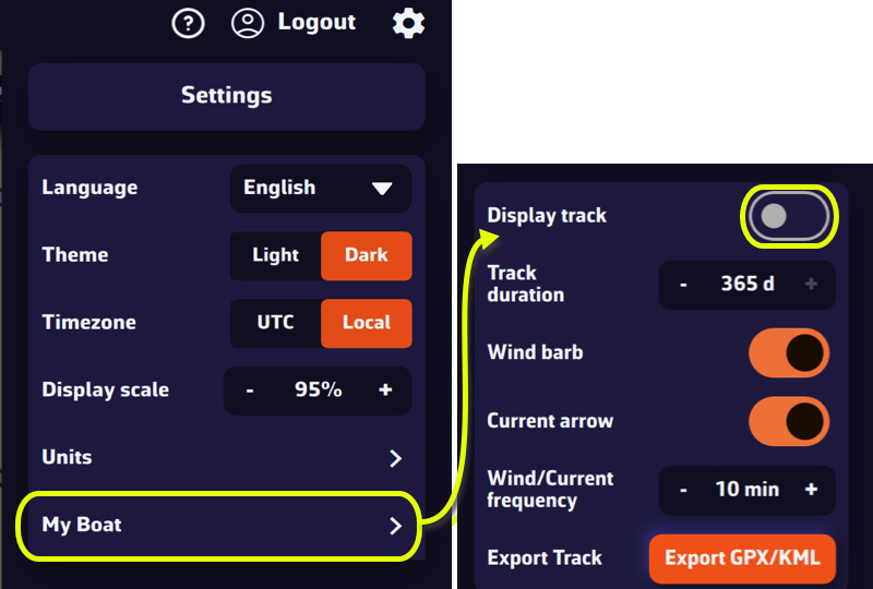
You are able to:
Procedure:
NavimetriX.exe file in its installation folder).By default, the target is placed in the center of the screen, allowing you to drag the map underneath it and use the zoom to position it at a specific location.
However, you can lock the target to other elements, or even disable it.

Tap/click on the layers button.
In the “Target” drop-down menu, select which element you want to lock the target to:
You can also lock the target onto a POI by editing it.
A GRIB file (for GRIdded Binary) is a standard file format used by meteorological services to distribute numerical weather forecasts.
It contains the raw data generated by weather models (wind, pressure, rain, waves, currents, etc.) organized on a grid covering a geographic area.
Why use this format?
What does a GRIB file contain?
Depending on the selected model, a GRIB file may include:
What is it used for in navigation?
A GRIB file allows you to visualize the evolution of the weather over a given area directly within your navigation software or weather app.
To illustrate the process, let’s say we’re planning a 4-day passage from La Rochelle (France) to Cowes (UK).
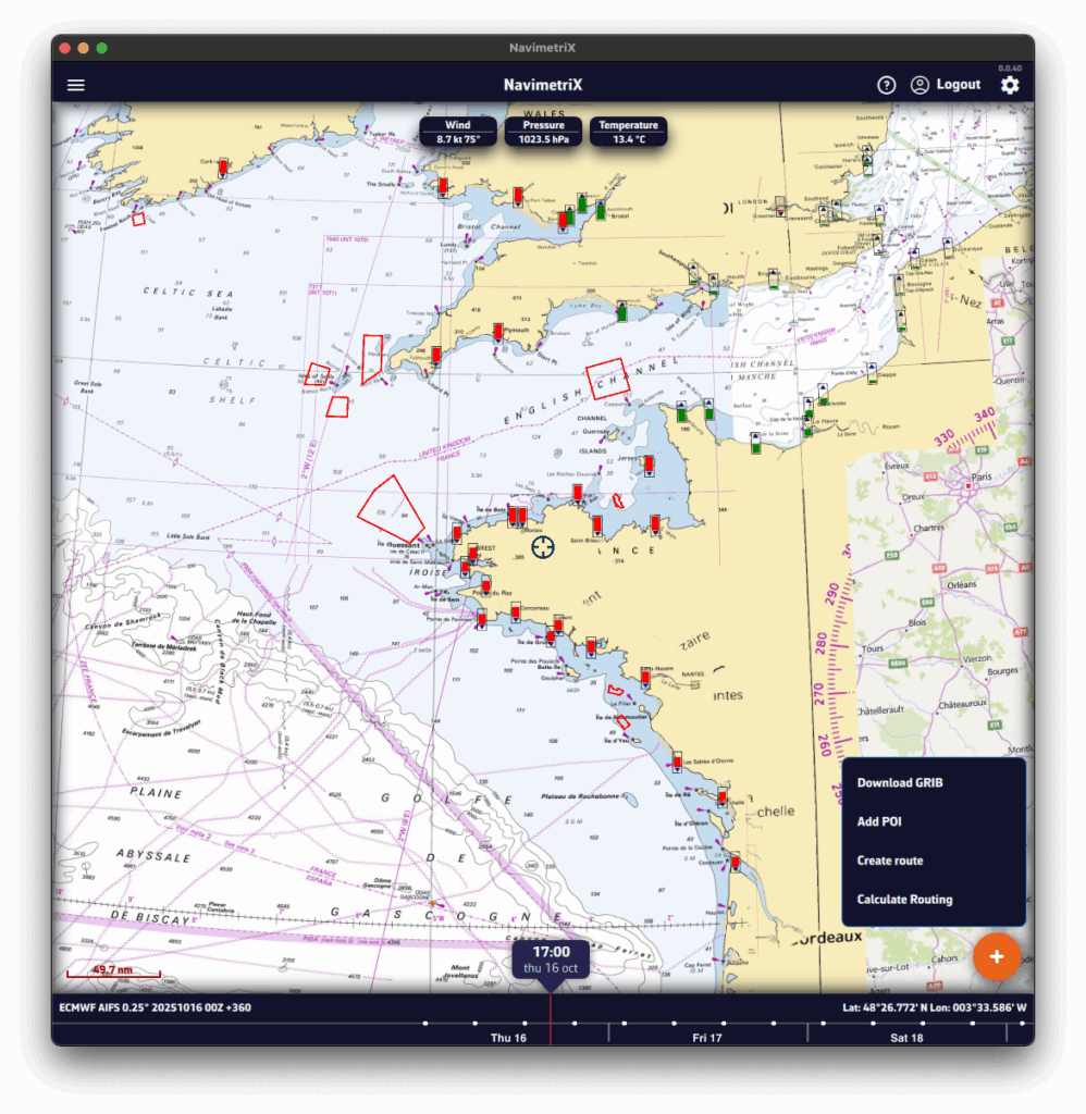
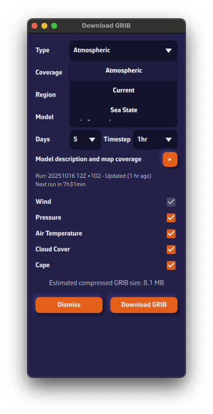
A Download GRIB window opens. The choices are filtered to your selected region.
Without the Premium option, you’re limited to the GFS model (the U.S. NOAA global atmospheric model).
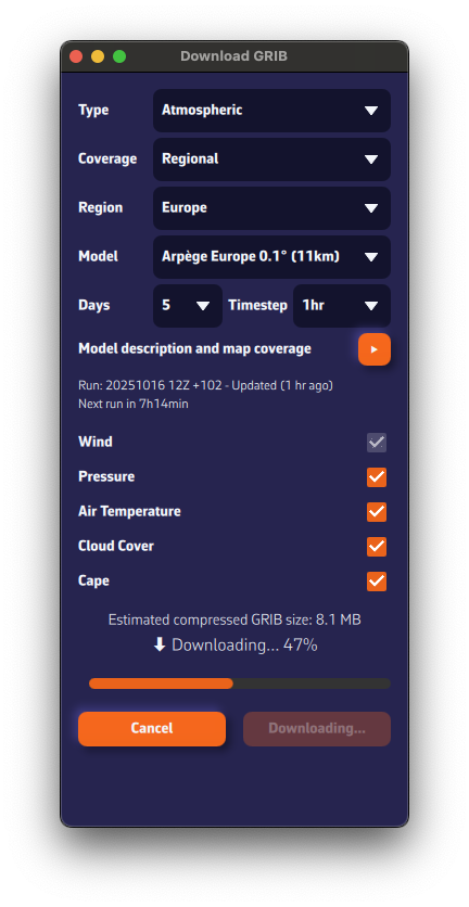
The estimated compressed GRIB size appears at the bottom. Keep it reasonable—if you see ~200 MB, you probably chose a model that’s too fine or too many parameters.
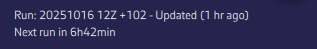
Below the model description, we show the latest model calculation time (the Run).Run: 20251016 12Z +102 means: calculated on Oct 16, 2025; initialized at 12:00 UTC (12Z); contains 102 forecast hours from that run.
We also display the estimated time until the next run is available.
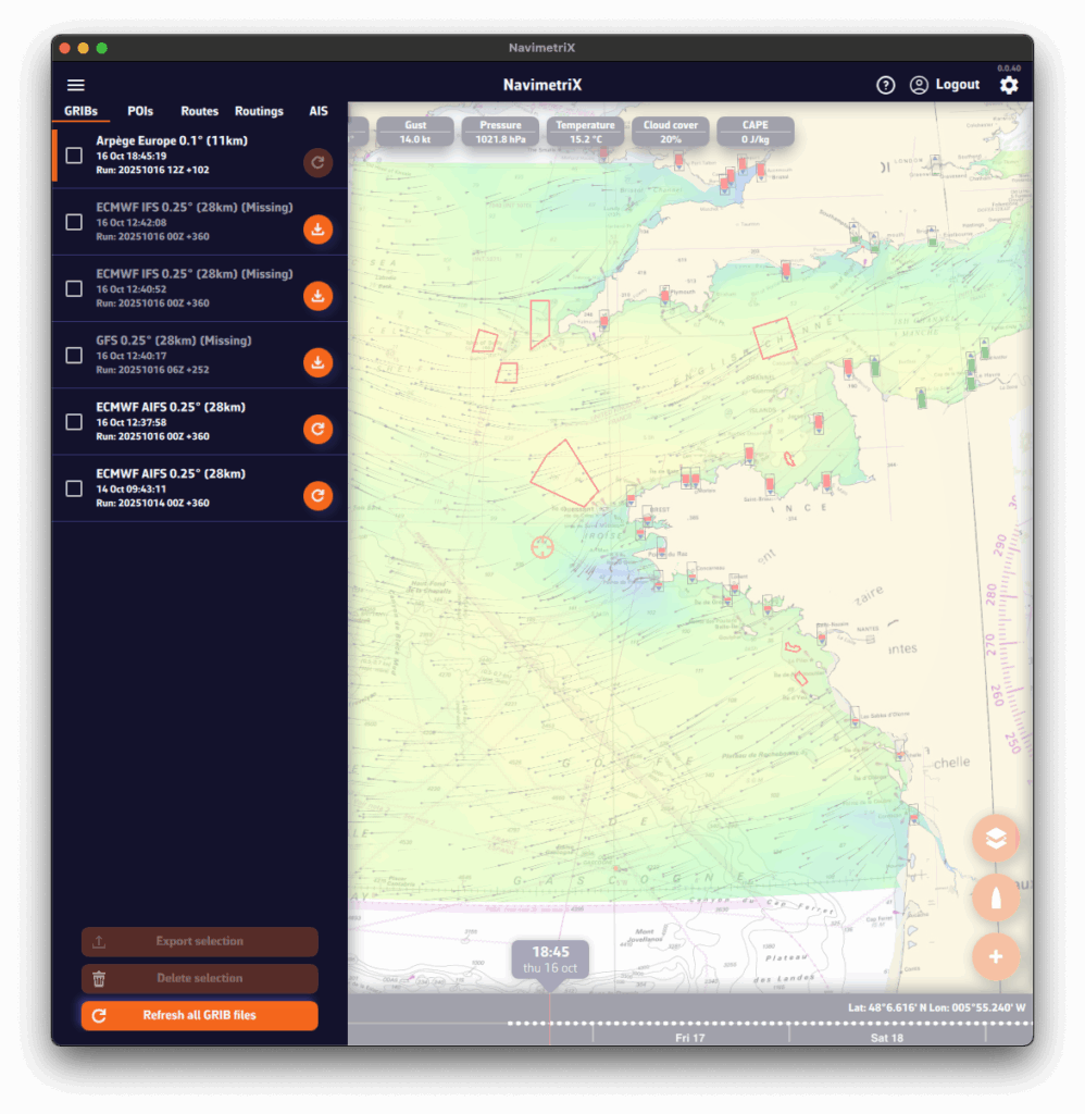
You may have noticed a small icon on the right of each item in the GRIB files list. This icon shows the update status of your GRIB file and can display three different states:
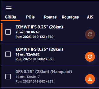
The icon appears in dark orange right after a GRIB file has been downloaded. This means your file is up to date — you already have the latest available version of the weather model.
This is what you will see immediately after downloading a GRIB file.
The icon turns light orange. This means a new model run (a new forecast) is available. To update your GRIB file, simply click or tap on this icon: the file will automatically be replaced with the latest version.
Finally, the icon may appear in light orange with a small download symbol. This means you have already downloaded this GRIB file on another device, but it is not yet available locally on the one you are using. To retrieve it, simply click or tap on the icon: the file will be downloaded automatically.
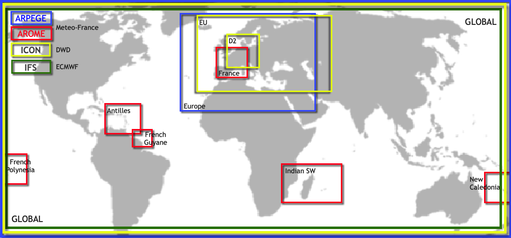
Global models (such as GFS or ECMWF) cover the entire planet. They are essential for long crossings and long-term forecasts (up to 10–15 days), but their resolution remains limited (20 to 50 km). They are used to get an overall view of the weather and for long-distance passages.
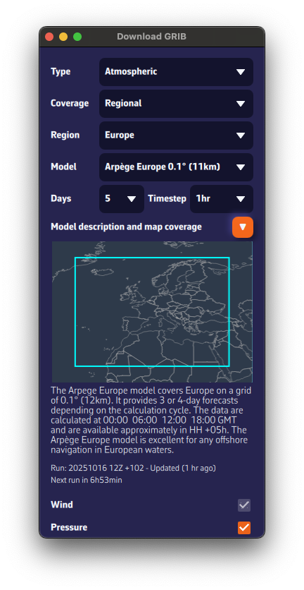
Regional models focus on a specific area (France, Europe, the Mediterranean…). Their coverage is smaller, but their resolution is much finer (2 to 10 km), allowing for better anticipation of local effects such as thermal breezes, thunderstorms, terrain, and coastal winds. In return, they generally only extend 2 to 3 days into the future. They are used for day trips or short cruises.
If you’re not familiar with weather models, you’re probably wondering which ones to choose.
Here are a few simple rules:
Select the model according to your navigation area and type of sailing, following the table below.
For weather data, if in doubt, choose the ECMWF IFS model.
The ECMWF IFS model covers the entire globe for up to 14 days. However, note that forecast reliability decreases with time:
| Forecast range | Reliability level |
|---|---|
| Up to 2 days | Excellent |
| 2–4 days | Very good |
| 4–5 days | Good |
| 5–8 days | Reasonable trend |
| 8–10 days | Rough trend |
| Beyond | At best a trend — often unreliable. Prefer the AIFS model, computed using Artificial Intelligence. |
Here’s a table to help you choose. We’ll soon add an automatic selection feature based on your sailing program.
| Type of data | Type of navigation | France – Atlantic & Channel | France – Mediterranean | Europe (outside France) | United States | Rest of the World |
|---|---|---|---|---|---|---|
| Weather | Day sailing in a bay | Arome | Arome | UKV, ICON, or Arpege Europe | Nam Conus Nest | ECMWF IFS |
| Weather | Coastal | Arpege Europe | Arpege Europe | UKV, ICON, or Arpege Europe | Nam Conus | ECMWF IFS |
| Weather | Offshore | ECMWF IFS and AIFS + GFS | ECMWF IFS and AIFS GFS | ECMWF IFS and AIFS GFS | ECMWF IFS and AIFS GFS | ECMWF IFS and AIFS GFS |
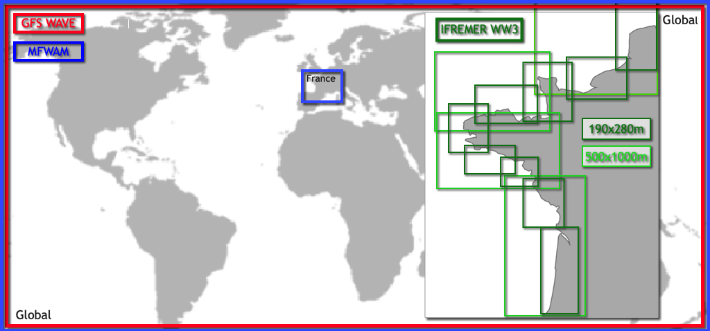
| Waves | Coastal | MFWAM France | MFWAM France | MFWAM | GFS Wave | GFS Wave |
| Waves | Offshore | MFWAM + GFS Wave | MFWAM + GFS Wave | MFWAM + GFS Wave | MFWAM + GFS Wave | MFWAM + GFS Wave |
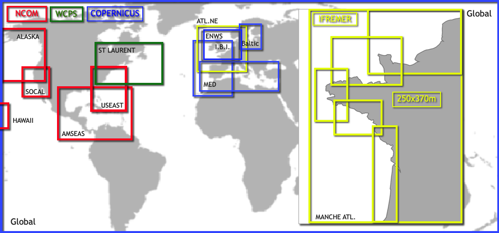
| Currents | Day sailing in a bay | Ifremer | Copernicus Med | Copernicus | MSC NCOM | Copernicus SMOC |
| Tidal currents | Coastal | Copernicus IBI | Copernicus Med | Copernicus IBI or ENWS | MSC NCOM | Copernicus SMOC |
| Ocean currents | All | Copernicus IBI | Copernicus Med | Copernicus IBI or ENWS | Copernicus Global | Copernicus Global |
These models provide a simplified description of the sea state.
In short, they include the significant height of the total sea, its period, its direction, as well as the same information for the wind sea.
They are mainly used in routing when conditions are challenging.
See also: It’s great to have all these models — but which one should I choose?
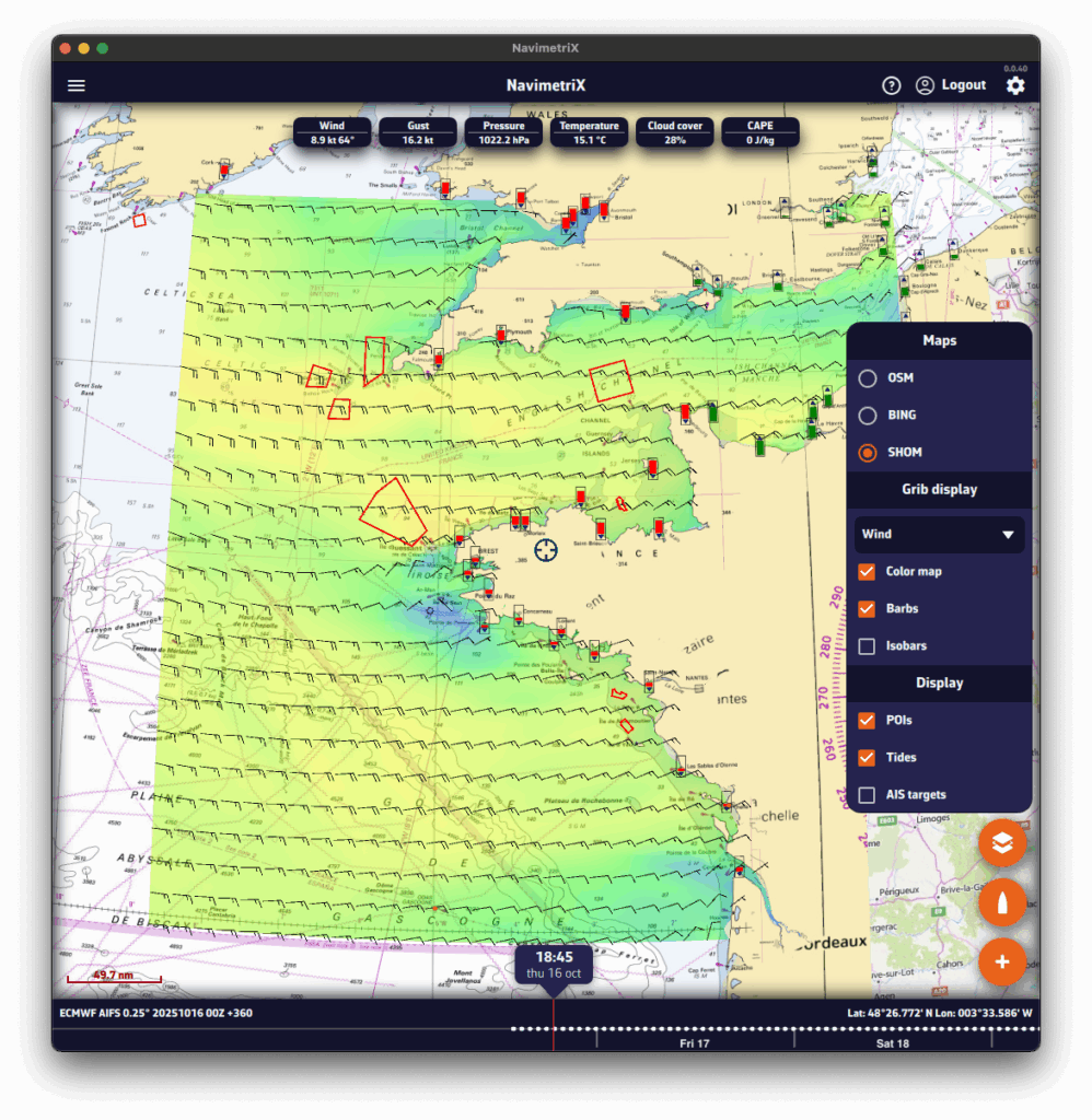
Open the Settings panel by tapping the cogwheel at the top right of the upper ribbon, then select GRIB Display.
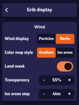
In the “Wind” section, select Particles or Barbs. Animated particles show the wind flow but consume more system resources and therefore battery — best avoided while sailing. Vectors and barbs are the classic meteorological representation of wind direction and strength. They are positioned on each grid point of the GRIB file and are more resource-efficient.
The Gradient style represents wind strength using a rainbow color scale — from blue (light or calm winds) to magenta (strong winds), through shades of green, yellow, orange, and red. Especially suitable for wind data.
The Isoplane style displays the data with the same colors but as equal-value zones. This style is better suited for data such as wave height, for example in 50-cm increments.
The Land Mask displays data over land as well. This is particularly useful when sailing among islands, to keep a continuous sea/land display.
Transparency allows you to adjust the color overlay depending on the background (satellite map or nautical chart).
The Iso-zone step adjusts the spacing between isoplane zones depending on the type of data (waves, precipitation, temperature, etc.).
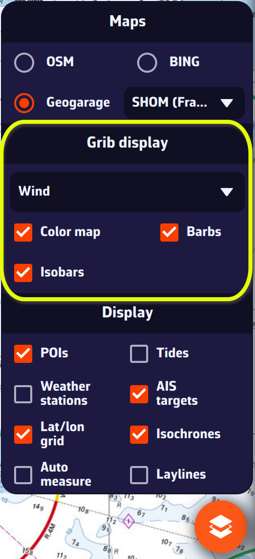
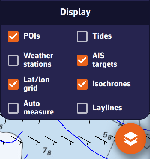
On the map, the Layer button at the bottom right of the screen lets you choose what to display.
In the GRIB Display section, the drop-down menu allows you to select which data to display. If a weather GRIB (for example an IFS model) is displayed, Wind will be selected by default. You can enable or disable the color background, particles or barbs (according to your previous setting above), and isobars (lines of equal atmospheric pressure).
If you have displayed a wave GRIB file, you can enable or disable the color background and the wave direction arrows.
This section automatically adapts to the type of GRIB file displayed on the screen: weather, waves, or currents.
By default, a tide gauge is displayed on the cartography for each referenced station.
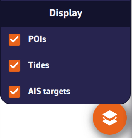
The display can be disabled by opening the layers menu and unchecking the Tide box. The gauges currently display dynamically:

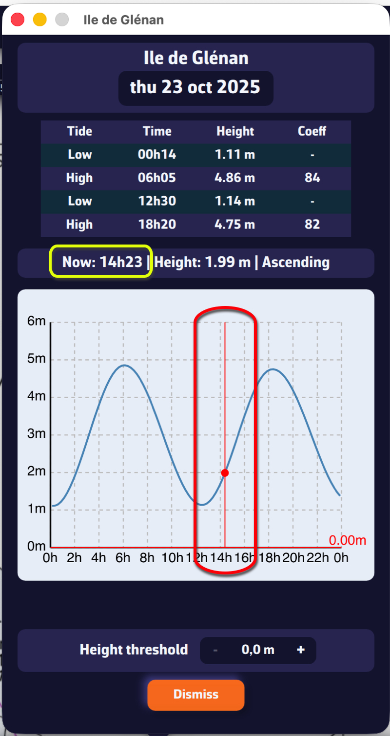
Tapping on each gauge opens a tide graph showing the tide curve and the current water level, represented by the vertical timeline.
The graph is topped by a table showing the times, water heights and tidal coefficients for the day.
Tapping/clicking on the date above the table opens the calendar, allowing you to select another day/month.
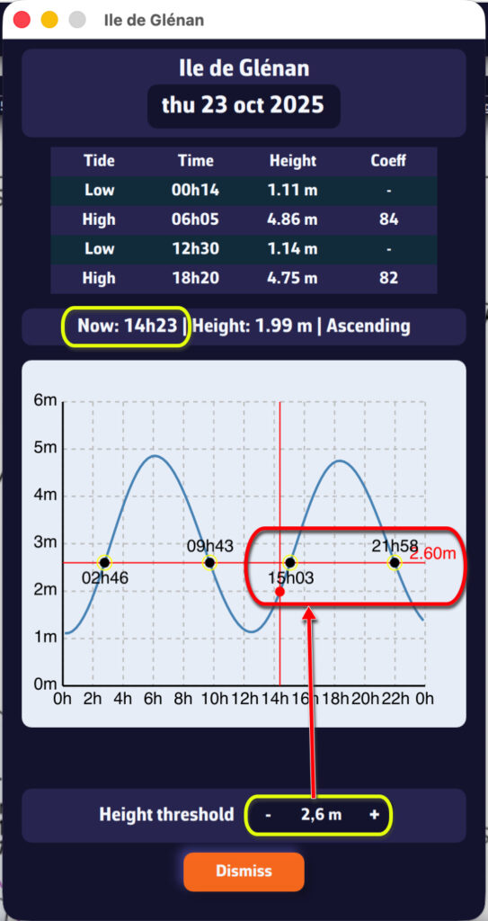
The height threshold can be used to determine:
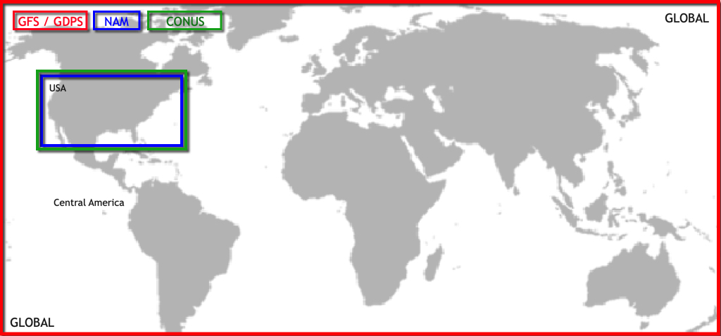
NavimetriX offers several high-resolution regional models for popular sailing destinations worldwide, in addition to global models like GFS, ECMWF, and ICON Global.
NAM (11 km resolution) — NOAA’s North American Mesoscale model covers the continental United States. Forecasts up to 84 hours with hourly time steps. Ideal for coastal navigation along the US East Coast, West Coast, and Gulf of Mexico.
HRRR CONUS (3 km resolution) — The High-Resolution Rapid Refresh model provides the finest resolution for the continental US. Forecasts up to 18 hours, updated hourly. Perfect for racing and detecting rapidly evolving conditions like sea breezes and thunderstorms.
Arome Antilles (3 km resolution) — Météo-France model covering the Lesser Antilles from Puerto Rico to Trinidad. Forecasts up to 48 hours. Excellent for inter-island passages and detecting trade wind variations.
Arome Guyane (3 km resolution) — Covers waters off French Guiana and the nearby South American coast. Forecasts up to 33 hours. Useful for sailors transiting between the Caribbean and Brazil.
Arome Polynésie (3 km resolution) — Covers French Polynesia including Tahiti and the Society Islands. Forecasts up to 48 hours. Ideal for detecting local effects around high volcanic islands and reef passes.
Arome Calédonie (3 km resolution) — Covers New Caledonia and the Coral Sea. Forecasts up to 48 hours. Essential for navigating the lagoon system and anticipating thermal effects around Grande Terre.
Arome Réunion-Mayotte (3 km resolution) — Covers the western Indian Ocean from the Mozambique Channel to the Mascarene Islands, including Madagascar, Réunion, Mauritius, and Mayotte. Forecasts up to 48 hours. Critical for this cyclone-prone region.
NavimetriX provides access to over 70 weather, wave, and current models from leading meteorological agencies worldwide.
GFS — NOAA — 28 to 222 km — 16 days
ECMWF IFS — ECMWF — 28 to 111 km — 15 days
ECMWF AIFS — ECMWF — 28 to 111 km — 15 days
ICON Global — DWD — 14 to 111 km — 5 days
Arpège Monde — Météo-France — 28 km — 4 days
GDPS (GEM) — CMC Canada — 17 km — 10 days
Arpège Europe — Météo-France — 11 km — 4 days
Arome — Météo-France — 3 km — 42 hrs
Arome HD — Météo-France — 1 km — 36 hrs
ICON Europe — DWD — 8 km — 5 days
ICON D2 — DWD — 2 km — 48 hrs
UKV — Met Office — 6 km — 5 days
NAM — NOAA — 11 km — 84 hrs
HRRR CONUS — NOAA — 3 km — 18 hrs
Arome Antilles — Météo-France — 3 km — 48 hrs
Arome Guyane — Météo-France — 3 km — 33 hrs
Arome Polynésie — Météo-France — 3 km — 48 hrs
Arome Calédonie — Météo-France — 3 km — 48 hrs
Arome Réunion-Mayotte — Météo-France — 3 km — 48 hrs
GFS Wave — NOAA — Global — 28 to 111 km — 16 days
MFWAM Global — Météo-France — Global — 11 to 56 km — 4 days
MFWAM France — Météo-France — France — 3 km — 4 days
IFREMER WW3 — Ifremer — France coasts (14 zones) — 190m to 500m — 4 days
Copernicus Global — Copernicus — 9 km — 5 days — oceanic currents only (Gulf Stream, etc.)
Copernicus Global SMOC — Copernicus — 9 to 56 km — 5 days
Copernicus IBI — Iberian-Biscay-Ireland — 3 km — 5 days
Copernicus ENWS — NW Shelf / North Sea — 2 km — 5 days
Copernicus BALTIC — Baltic Sea — 4 km — 5 days
Copernicus MED — Mediterranean — 5 km — 5 days
SHOM Manche-Gascogne — Channel & Biscay — 2 km — 5 days
SHOM Méditerranée Nord — NW Mediterranean — 2 km — 5 days
IFREMER — France coasts (10 zones) — 250m to 3 km — 4 days
MSC Saint Laurent — St. Lawrence / Atlantic Canada — 1 km — 84 hrs
NCOM Alaska – N. Calif — Alaska to N. California — 4 km — 90 hrs
NCOM Caribbean — Gulf of Mexico & Caribbean — 3 km — 90 hrs
NCOM Hawaii — Hawaii — 4 km — 90 hrs
NCOM South California — Southern California — 4 km — 90 hrs
NCOM US East Coast — US East Coast — 4 km — 90 hrs
In order to rename a GRIB file, you must click/press and hold on its name. This will bring up the keyboard, allowing you to change the name:
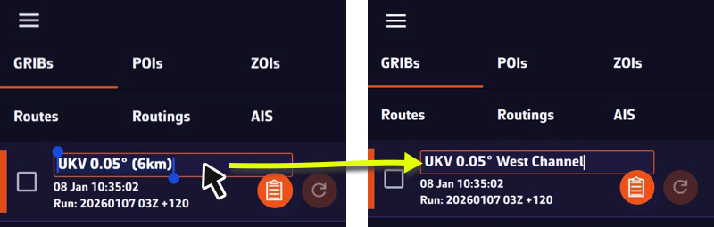
The name will be preserved during updates and synchronization.
The term “waypoint” doesn’t exist in NavimetriX. Instead, we use POI (Point Of Interest), a more generic term that can include many elements (targets, anchorages, beacons, race marks, etc.).

Drag the map under the target on the screen, zooming in to position it accurately.

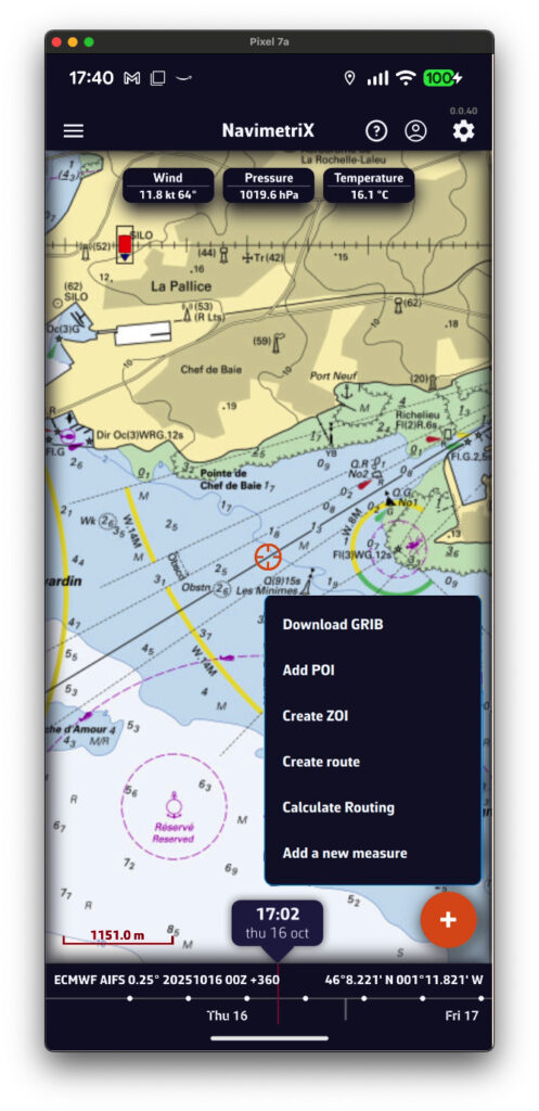
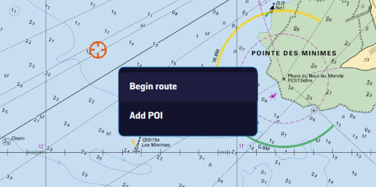
Tap the + icon in the bottom right corner of the screen and select ‘Add POI’ from the menu.
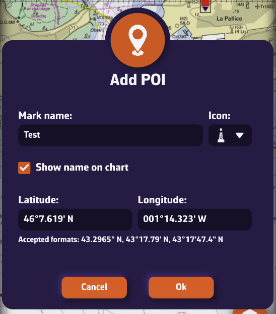
Tap OK to confirm.
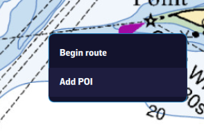
Place the mouse or trackpad pointer on the desired location on the map, without worrying about the target, and right-click. In the popup that appears, select “Add a POI”. The creation window opens as shown here.
Alternatively, you can proceed the same way as on a tablet or smartphone.
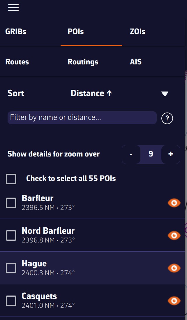
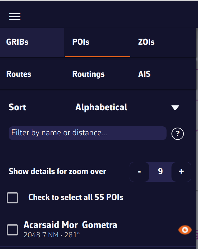
The points are saved in the POI list, located in the left sidebar of the screen, accessible via the ≡ symbol in the top-left toolbar.
You can show or hide each point individually by tapping the eye icon on the right side of the column.
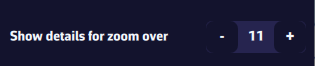
You can adjust the display so that the name and optional icon appear only from a certain zoom level, preventing the map from becoming overloaded if you have many points.
Move the chart under the target displayed on the screen, zooming in for precise positioning, then tap the + icon in the lower right corner. From the menu, select “Create a route”.
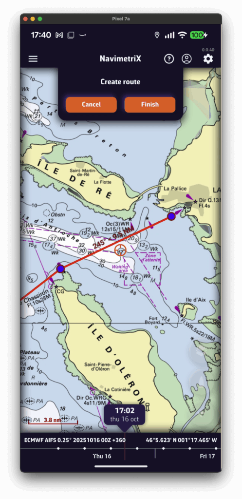
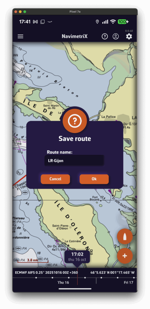
Tap successively to place the desired points. You can drag them with your finger to move them if needed. Zoom in for more precise placement. Once finished, select the “Finish” button at the top of the screen. Enter a name for your route and confirm saving by tapping “OK”.
Click to create successive points, zooming in for better accuracy. You can also drag the points to adjust their position if needed. Click the “Finish” button at the top of the screen. Enter a name for your route and confirm saving by clicking “OK”. Alternatively, you can proceed the same way as on a tablet or smartphone.
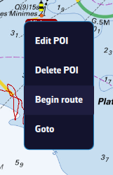
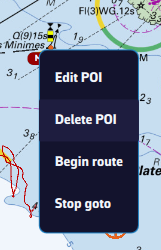
In any case, you can also create a route by tapping or clicking an existing POI (waypoint) and selecting “Begin route” from the popup menu starting from that point.
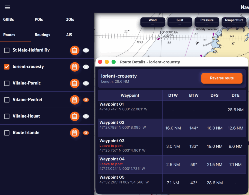
Routes are saved in the Routes list, located in the left sidebar of the screen, accessible via the ≡ symbol in the top-left toolbar.
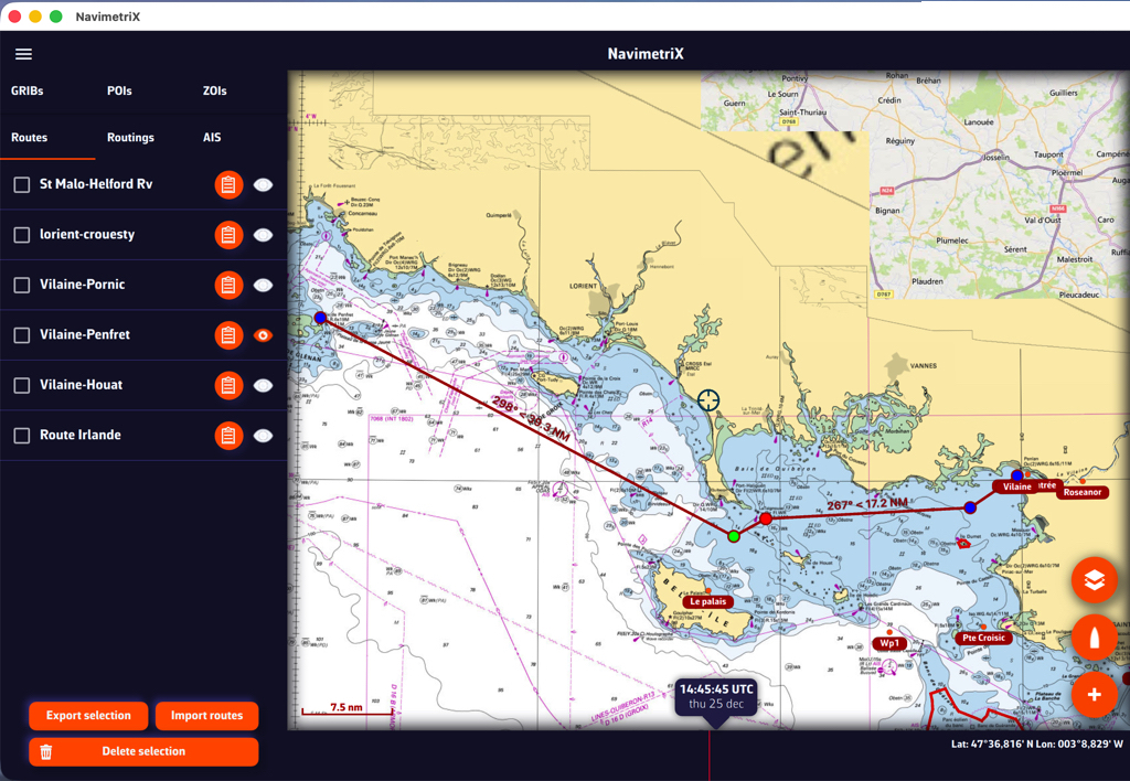
Tap the “eye” icon next to each route to toggle its display on or off. Use the checkboxes to select routes for export or remove.

A “Table” icon allows you to open the detailed route info. Tap/clic “Reverse route” button to sail back.
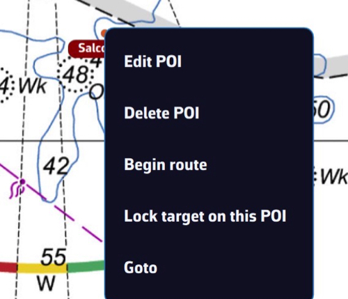
Tap or click, depending on your device, on a POI, and in the menu that appears select “Edit POI” to open the edit window.
See also: How do I create a POI or waypoint
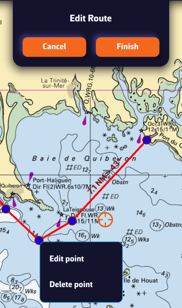
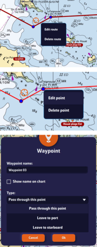
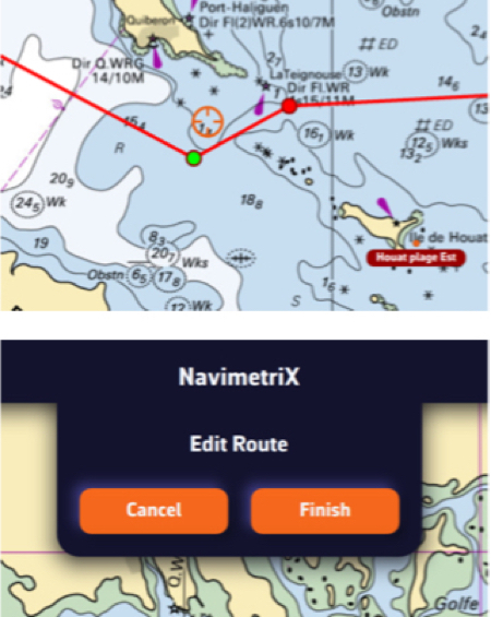
Open the left sidebar and select the “Routes” section. Display the route on the map by activating the “eye” symbol, then tap or right-click (depending on your device) on any part of the route. In the menu that appears, choose the option “Edit route”.


You can then drag points on the map to move them, add new ones by tapping on a segment of the route, and edit or delete any existing route point.
See also: How do I create a route?
To start navigation toward a POI (or Waypoint):
💻 On a computer: right-click the waypoint you previously saved, then select Go to. Confirm that you want to navigate to this waypoint.
📱 On a mobile device or tablet: tap the POI, then select Go to and confirm navigation.
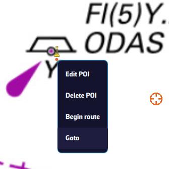
Once the POI is selected, if the boat (the GPS) is at sea, a black dashed line is drawn between your boat and the POI.
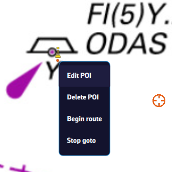
To stop navigation, tap or click again on the POI you are navigating to, then choose Stop goto from the menu.
Your boat’s polar determines all routing calculations. It represents your boat’s performance depending on wind speed and angle.
The application supports files in the .pol format (also used by Weather4D, SailGrib, Adrena, and others).
To choose your boat’s polar from the library:
Most of these polars come from naval architects or ORC certificates.
To find your polar, you can:
Once you’ve found your polar, select it and it will be confirmed.
Comment importer une polaire?
The application can import polars in the .pol format.
To import your own polar:
iPolar lets you create a polar in one minute based on your boat’s characteristics:
Note: The iPolar method was developed by KND, experts who work with the America’s Cup, TP52s, and IMOCAs — the best in their field!
Some polars are formatted as .CSV (Comma Separated Value) files, where the field separator is a comma or semicolon. This format is not supported in NavimetriX, unlike the .POL format where fields are separated by tabs — a format widely used in navigation applications. Therefore, you need to convert your .CSV file to .POL.
Open a new Excel sheet and select the menu: File > Import.
Choose “CSV File” and then select your polar file from the Finder.
Check the box Delimiters = “Semicolon”, then insert the data into the existing sheet.
Then save the file in “Text (Tab delimited)” format, which will create a .TXT text file.
Finally, rename the file by replacing the .TXT extension with .POL:
Your polar file is now ready to be imported.
Open the .CSV file with Numbers:
Export the file to TSV:
Replace the file .TSV extension to .POL, that’s all.
To compute a routing, you must first have:
Once these 3 steps are done, you can compute a routing by pressing the “Compute routing” button.
Remember: a routing is only useful if it’s correctly calibrated and you understand the computed result. Doing a single run and treating it like a train timetable will, at best, lead to disappointment.
We therefore recommend this approach:
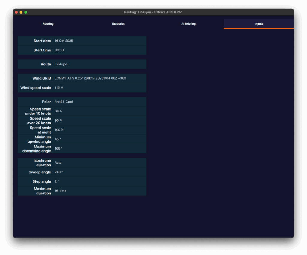
Click the “+” button, then select “Compute a routing”. A screen titled Routing opens.
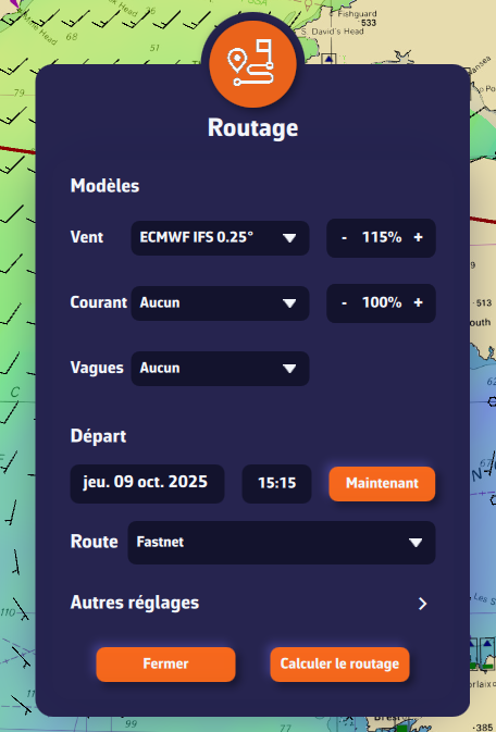
You can choose three forecast models:
To begin, select only a wind forecast file.
We recommend setting the wind factor to 115%. This means taking 115% of the wind speed from the GRIB, reflecting that GRIB wind speeds are often lower than reality.
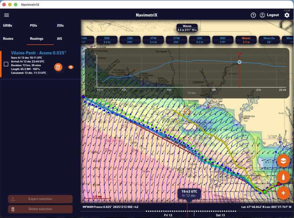
In a second step, following our recommendations, select a current model and a wave model.
Click the date to open the calendar and select your departure date. Click OK.
Click the time to open hour/minute selection, then also validate with OK.
Select the route you just created.
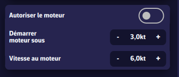
These are less frequently modified, but here are the main parameters at a glance.
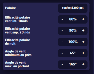

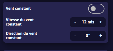
Useful for studying, for example, the effect of current in a bay. It freezes the wind (e.g., as measured at the masthead) to understand the current’s influence on the optimal route.
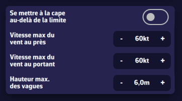
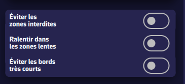
Allows you to constrain the optimal route. Use with care, otherwise the routing may not converge. For example, don’t set a max downwind wind speed of 20 kn for an ocean passage.
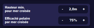
We define a cross sea when the angle between total sea direction and wind sea direction is between 45° and 135°. If the total sea height is high enough, the boat is significantly slowed. You can set the slowdown parameters here.

It’s easy to get a bit lost among all these settings. The default values were chosen carefully. Press this button to restore them.
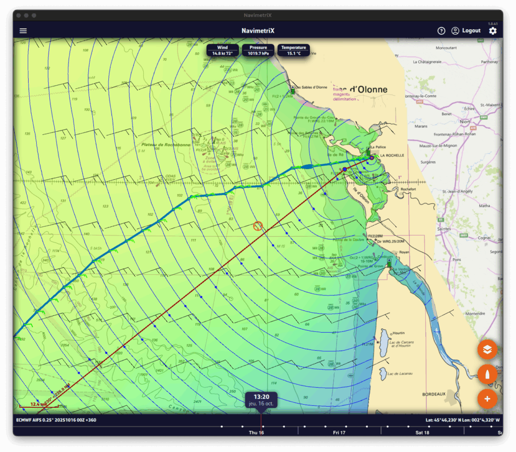
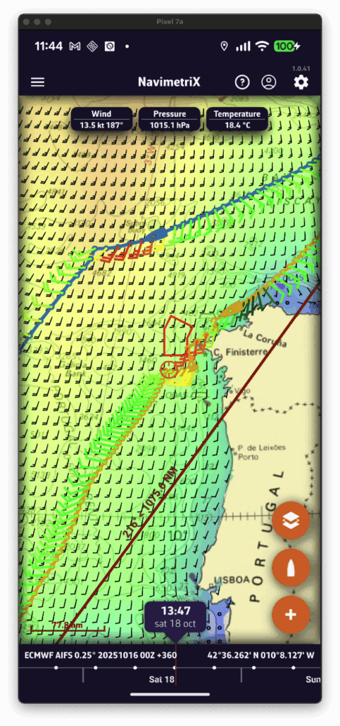
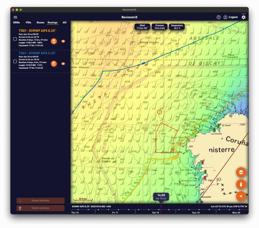
Once the routing is computed, the optimal route is shown on the chart together with the isochrone curves. These curves represent the positions that can be reached at successive time intervals from the start point.
You can move the boat along the route in two ways:
At each intersection between the optimal route and an isochrone, a wind barb is drawn. It shows the wind speed and direction at the time the boat reaches that position. If you route with current, a current arrow will also be drawn
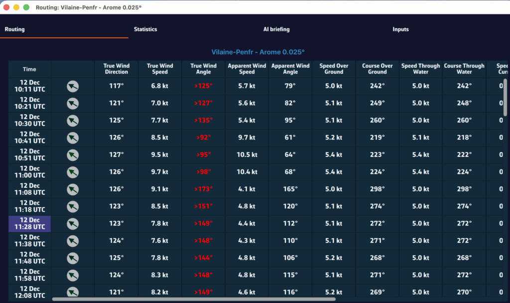
Open the lists panel (via the ☰ button at the top left of the screen) and select the Routing tab. This tab lists all computed routings.
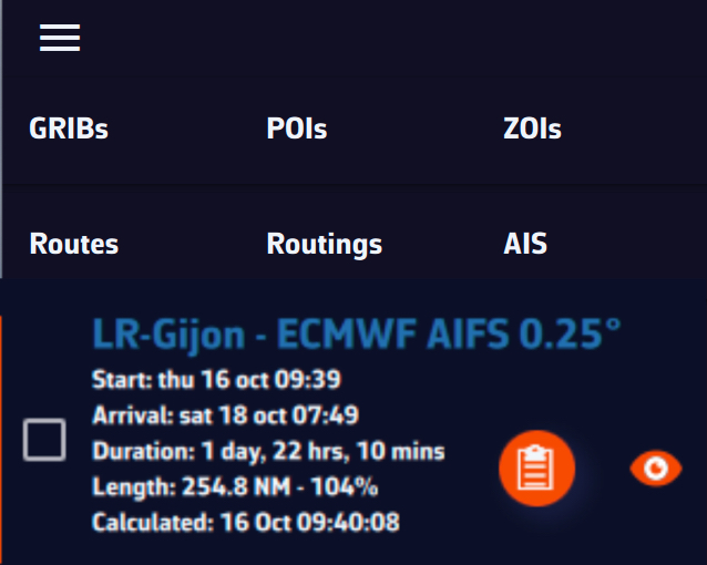
For each routing you’ll see:
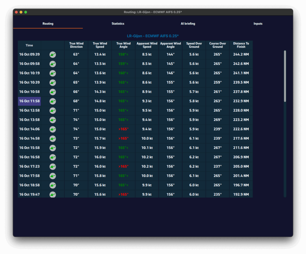
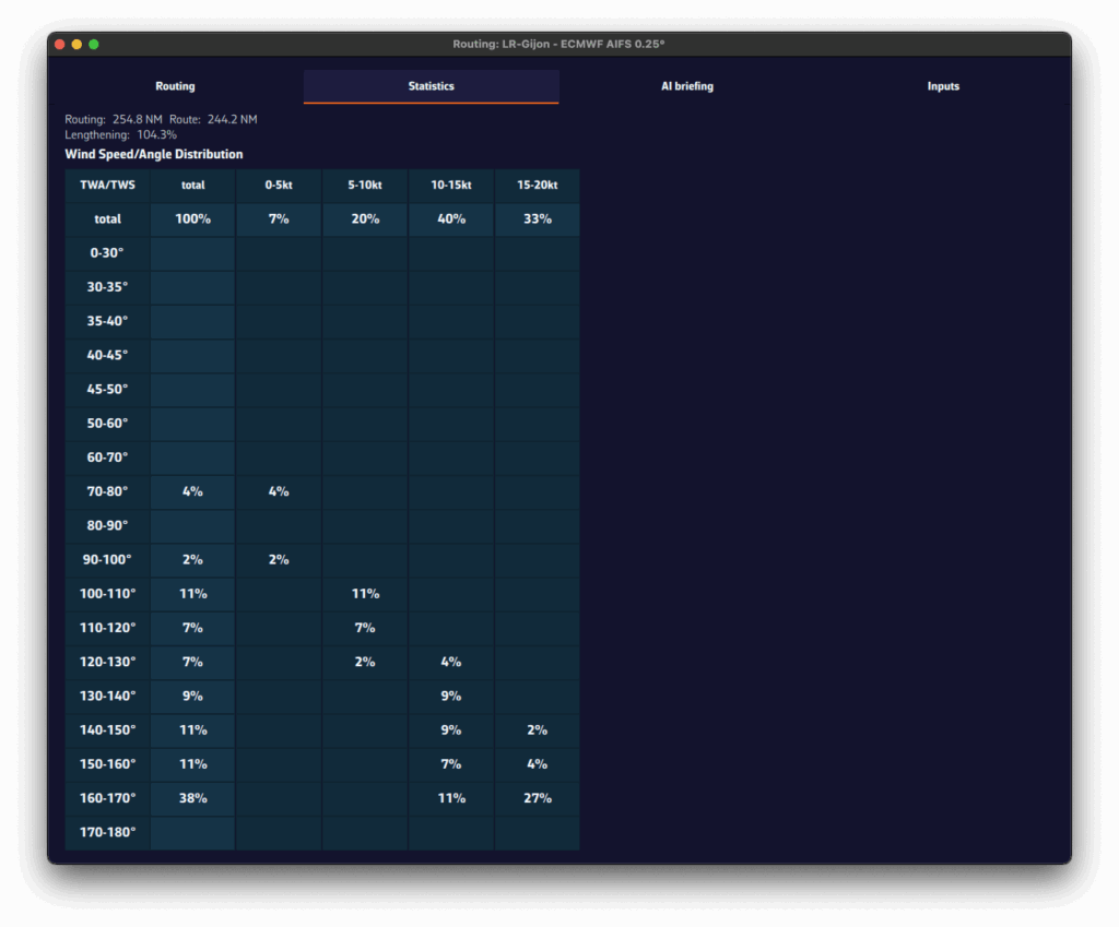
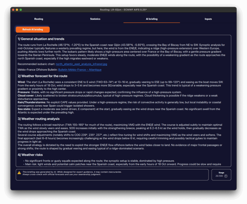
Click the orange button to open the routing table. It contains four tabs, each presenting a different facet of the computation.
A pivot point is a location you want the routing to pass through.
It’s a very useful way to quickly compare routing options.
For example, in this case we’ll check whether it’s better to pass inside or outside the Traffic Separation Scheme (TSS) off Cape Finisterre — a very common situation when sailing from the French Atlantic coast toward Madeira or the Canary Islands.
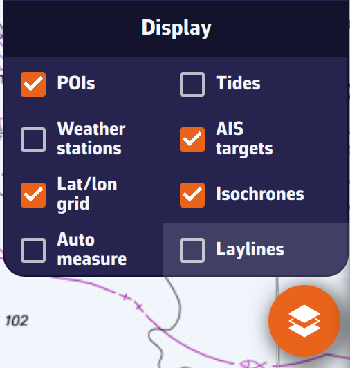
To perform a routing with a pivot point, first make sure the isochrones of the desired routing are displayed on the map.
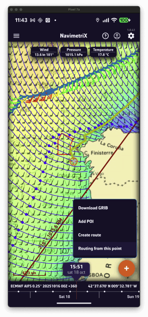
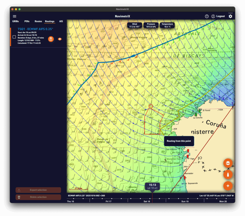
First you have to verify that Isochrones are checked in the Display section of layers menu:
Then simply tap/click on the name of the routing in the sidebar:
When isochrones are displayed, you can use a pivot point.
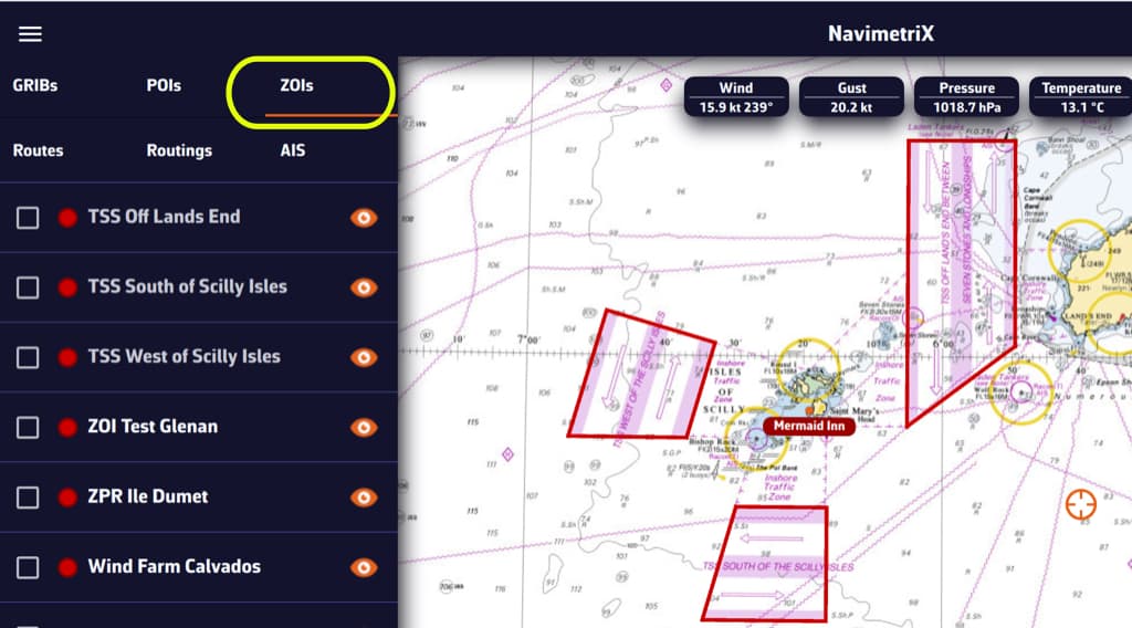
ZOIs are areas to avoid or areas of particular interest. Some are pre-existing in the application, but you can create as many as you need. There are three types:
Only no go zones and slow zones are considered by the routing calculation, if they are displayed on the chart. In the left side menu list, you can enable/disable the display of a zone on the chart by tap/click on the eye icon, select one or more zones to export or delete them by checking the box(es). You can also import ZOIs.
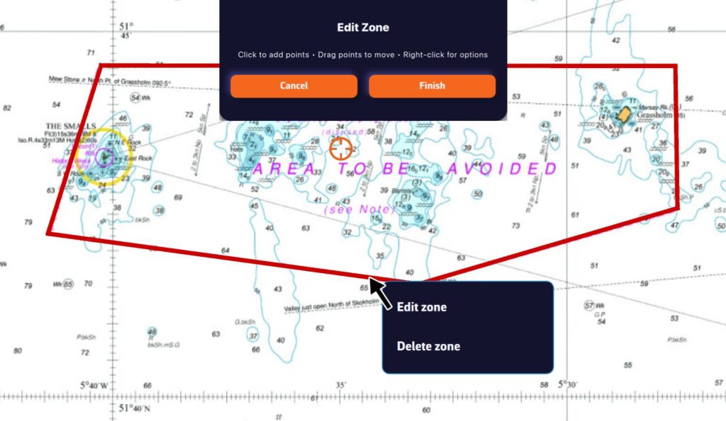
Tap/click on the border of a ZOI to edit/delete it. You can move the borders by selecting the corners, add an intermediate point anywhere on the border to modify it. After selecting the ‘Finish’ button, you can also change the name and type of the zone.
When isochrones are displayed, data labels in the same colour as the routing boat allow you to track progress along the route. In addition, clicking/tapping on each label displays the data graph from the start to the end of the route.
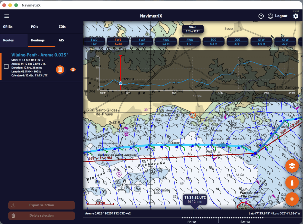
To scroll the boat along the route, a weather model must be displayed to activate the timeline.
A routing table is generated automatically and appears as an icon next to the route. Simply tap/click on the icon to display it.
Today, marine charting compatible with the app is provided exclusively by the Geogarage platform, where you must create an account and subscribe to one or more chart services depending on your sailing areas.
The charts available come from the official digital data of many international hydrographic offices such as the SHOM, UKHO, NOAA, and others.
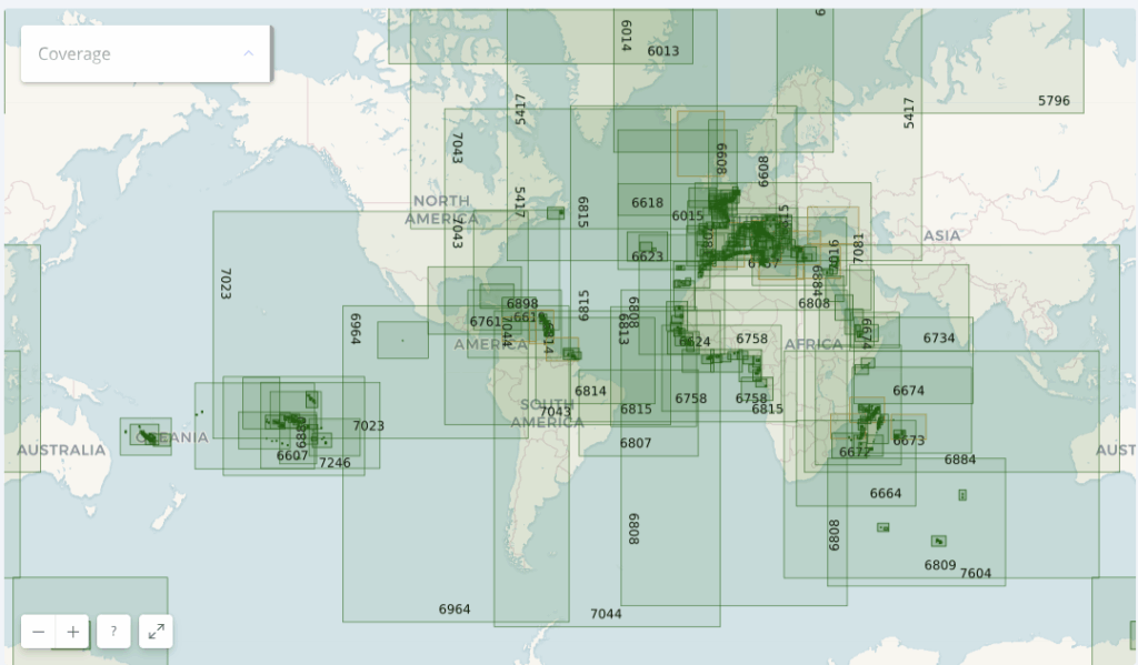
Currently, about thirty publishers are available, offering near-global coverage. These are raster charts divided into tiles, allowing smooth zooming between scales.
When you subscribe to a hydrographic service via Geogarage, you gain access to all the charts published by that hydrographic office.
For example, if you subscribe to the SHOM (Service Hydrographique et Océanographique de la Marine) charts, you will have access to all SHOM charts.
Thus, if you’re sailing from La Rochelle to Fort-de-France across the Atlantic, a single SHOM chart subscription is probably sufficient to cover your entire passage.
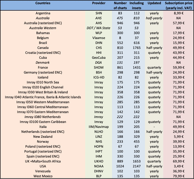
As a reference:
Below is an illustration showing the diversity of hydrographic services available through Geogarage:
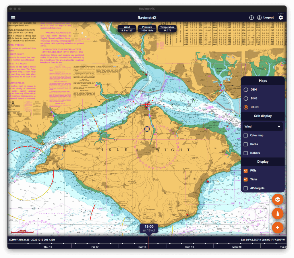
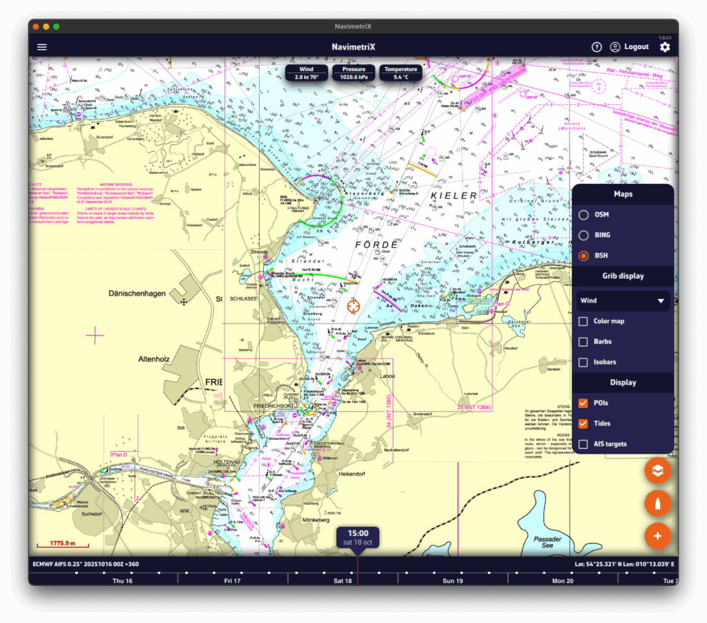
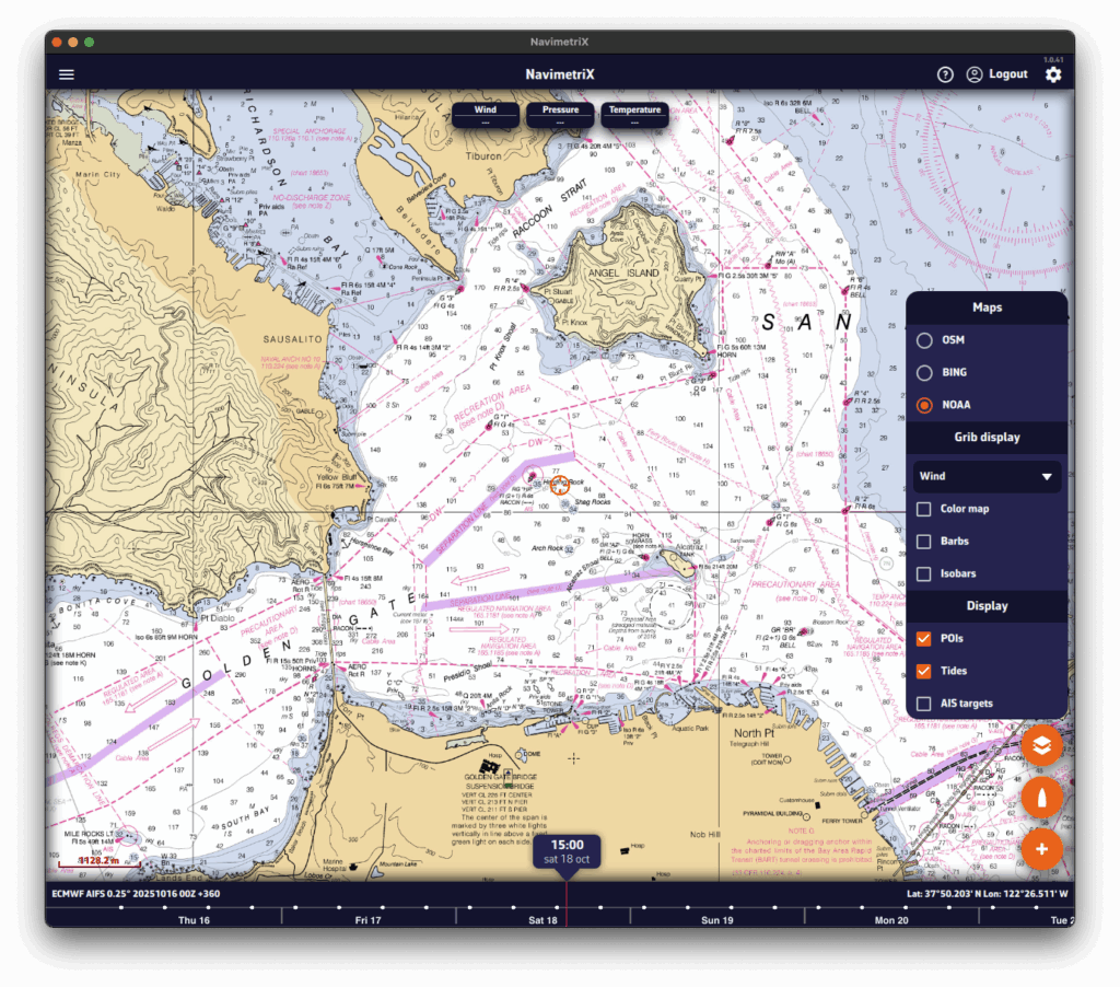
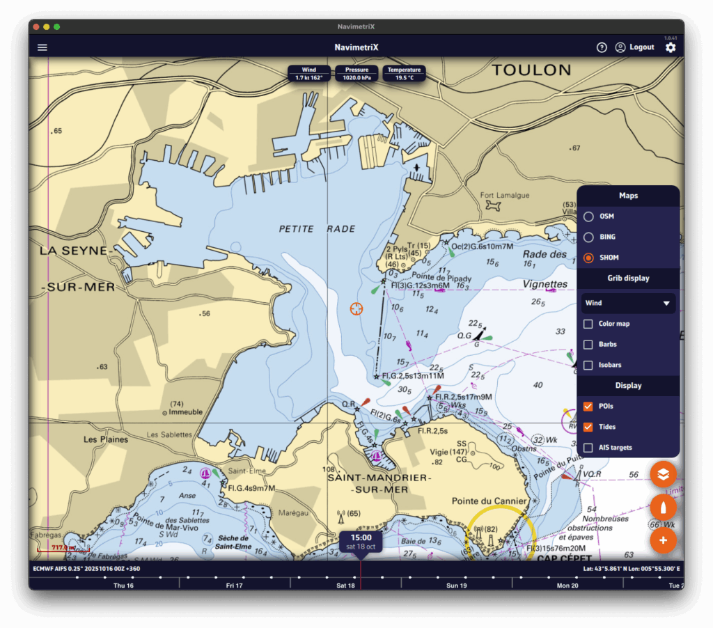
Select a hydrographic service to view the chart coverage included with that subscription.
Annual subscription prices (VAT included)
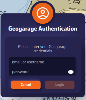
In the Settings of Navimetrix, under the Geogarage Charts menu, you need to log in by tapping the “Login” button and entering your Geogarage account credentials.
Once connected, select your subscribed chart service (for example UKHO) from the “Layer” dropdown list. The chart display updates instantly while connected to the internet.
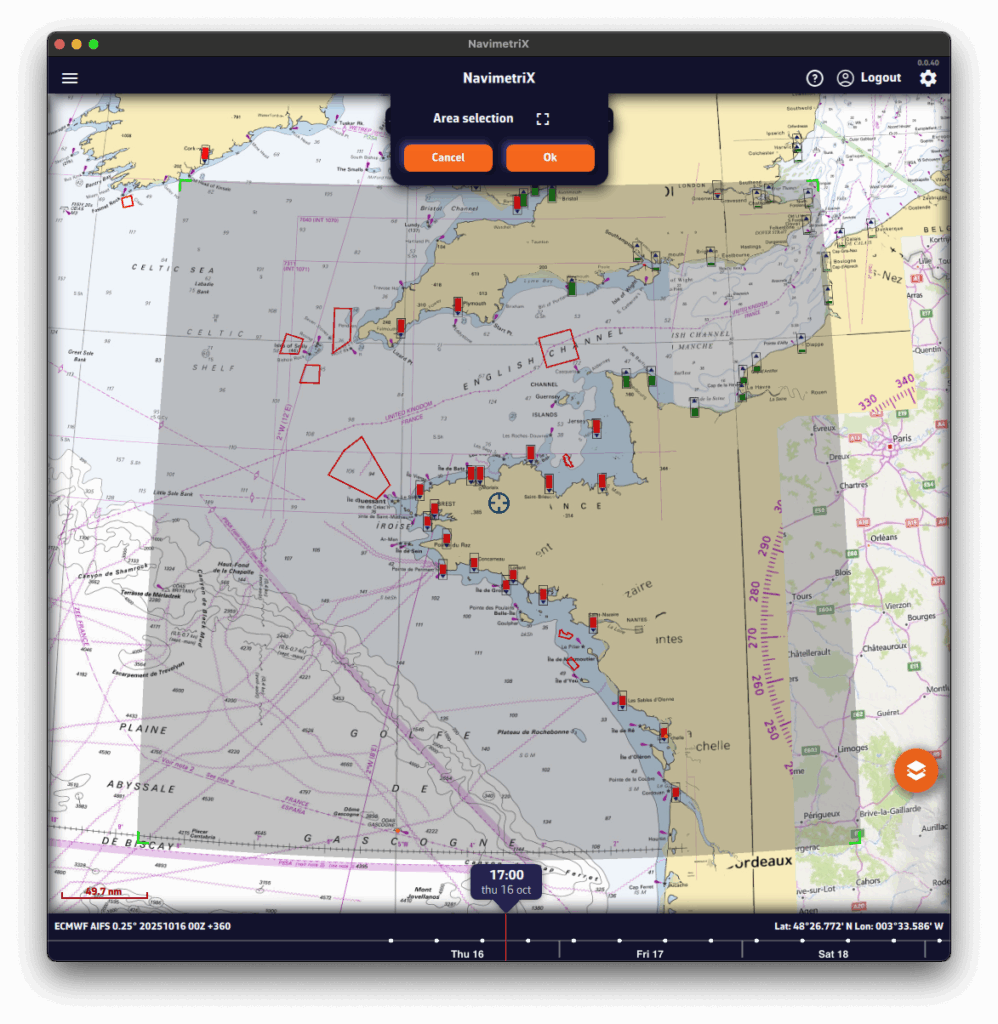
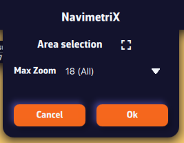
In the Settings of NavimetriX, under the Geogarage Charts section, tap “Add New Zone”, then define the geographical area to download by dragging the green corners of the grey rectangle.
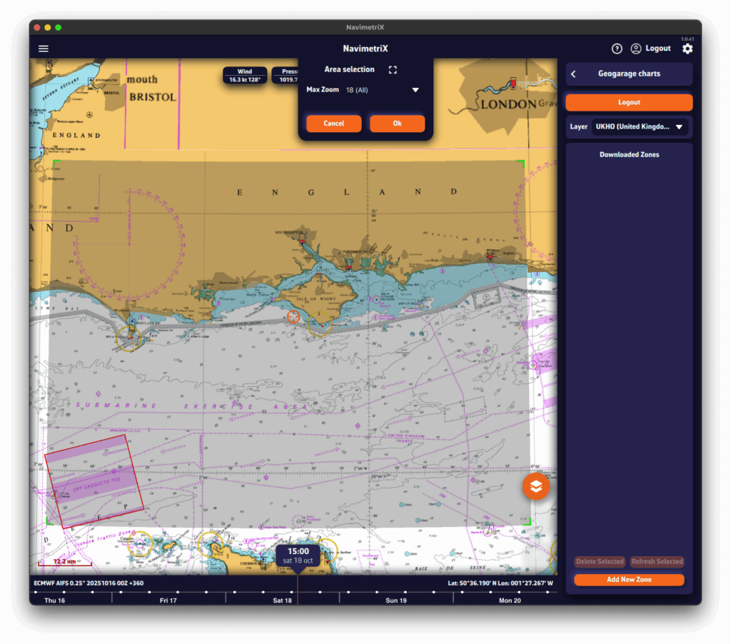
The Area selection dropdown menu offers two zoom-level options for the maximum chart scale:
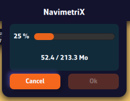
Once confirmed, a countdown shows the preparation and download progress.
A green frame remains visible so you can add new adjacent download zones without overlap using the “Add a new area” button. Only downloaded charts are available for offline use.
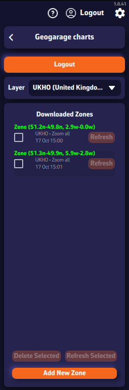
The downloaded chart zones are listed by publisher in the Geogarage Charts drawer. A checkbox allows you to select them for the Delete or Refresh functions.
Whenever a chart update is published by the provider, the Refresh button next to each zone becomes active. You can update them individually or in bulk by checking multiple boxes and pressing “Refresh Selected”.
In order to rename a chart area, you must click/press and hold on its name. This will bring up the keyboard, allowing you to change the name:
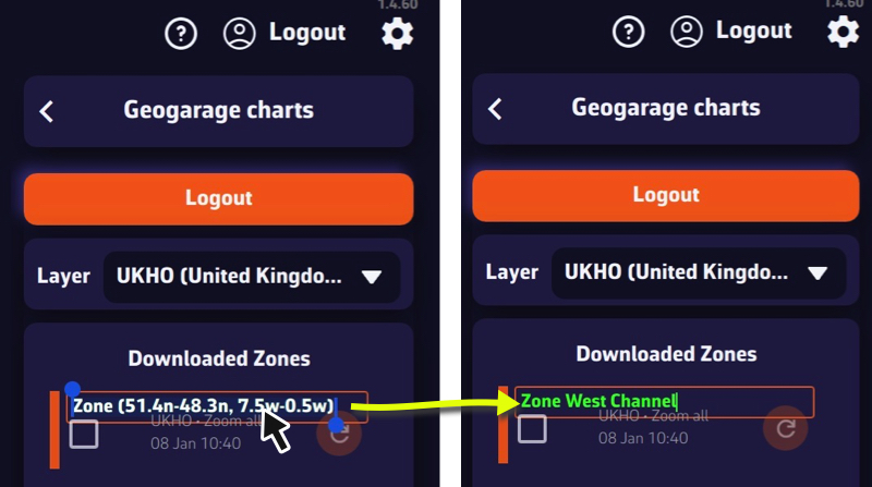
The name will be kept during updates and synchronization.
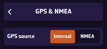
While sailing, if you want to display your phone’s GPS data, open the app settings (gear icon in the top-right corner).
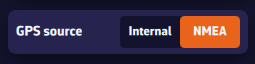
Go to the GPS & NMEA menu and make sure the GPS source is set to Internal.
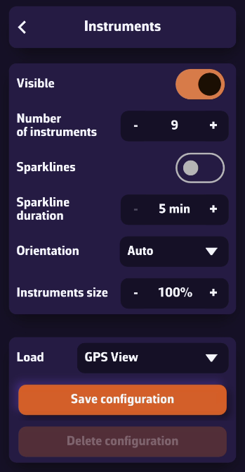
Exit this menu, then open Instruments. Check the Visible box to show the instruments, and make sure the selected layout is GPS View.
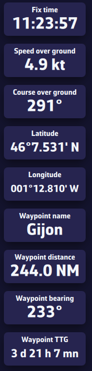
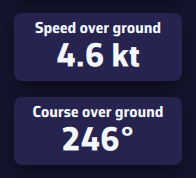
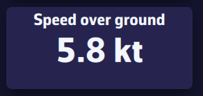
Once your phone receives a GPS signal, the time of the last position, your speed over ground (SOG), and your course over ground (COG) will be displayed in the instrument bar.
You can scroll through the parameters to view your coordinates and POI data if you’ve selected a waypoint using the Go to function.
On phones, the default display is horizontal.
On tablets or computers, the layout automatically adjusts to a vertical view.
To activate navigation toward a POI (or Waypoint):
💻 On a computer: right-click the waypoint you previously saved, then select the Go to option. Confirm that you want to navigate to this waypoint.
📱 On mobile or tablet: tap the POI, then select Go to and confirm the navigation.
Once the POI is selected, a dashed black line is drawn between your boat and the POI, showing the direct route.
To stop navigation, select the same POI again, then choose Stop Goto from the menu.
Not yet. USB GPS receivers are not currently supported directly by the application.
For now, only GPS devices transmitting NMEA data over Wi-Fi are compatible.
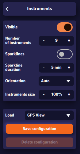
To change the displayed instruments, open the right panel using the gear button at the top right of the screen, then select Instruments.
You will see several settings:
On a computer, right-click an instrument. On a mobile device, perform a long tap.
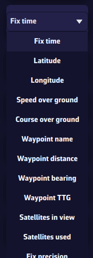
A list of parameters appears — select the one you want to assign to that instrument.
To save a configuration, press the Save Configuration button, enter a name, and confirm to save it.
Saved configurations are specific to each device — they are not synchronized between your phone and your computer, ensuring optimized layouts for each screen.
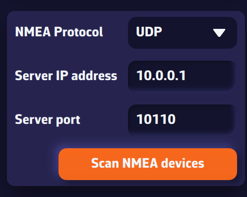
To receive NMEA data from your onboard instruments:
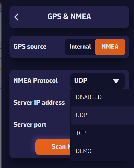
The first line corresponds to the GPS source. If you want to receive GPS data through an NMEA stream, select NMEA.
If you don’t know these values, press Scan for NMEA Streams. The scan will automatically search for known configurations. When a stream is detected, NavimetriX will offer to apply the parameters automatically (protocol, IP, port). Select Yes and close the scanner — your NMEA source is now active!
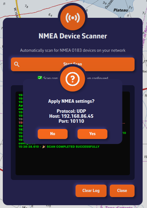
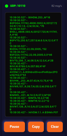
Once connected, NMEA data appears in green in the log window at the bottom of the panel.
If no stream is found, enter your NMEA system parameters manually. We recommend using the UDP protocol for maximum flexibility.
The last section lets you enable NMEA logging. When enabled, all received NMEA sentences are recorded. You can set a retention period (for example, 8 days) and specify when the logs should be compressed. Uncompressed daily files can be large (around 60 MB), but once compressed, they are only about 10% of their original size.
The Export Logs button allows you to save these files for analysis or replay with external tools such as VDR Player.
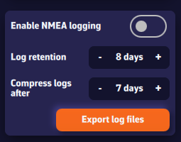
Note: A built-in feature to replay NMEA logs will be added in a future version of the app.
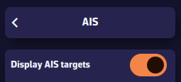
Prerequisite: make sure your NMEA stream is properly configured and that you are receiving AIS sentences (they start with AIVDM).
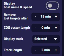
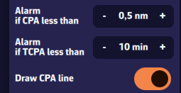

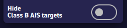
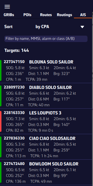
You can hide Class B AIS targets (small recreational boats) to show only Class A (cargo, ferries, etc.)—useful at crowded race starts.
Open the hamburger menu (☰ top left) and choose the AIS tab to display the target list.
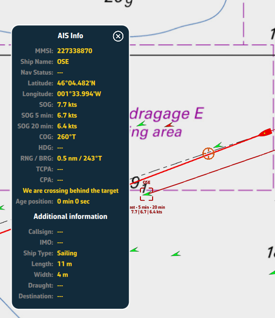
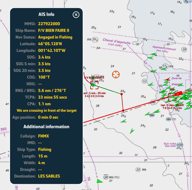
For each AIS vessel, the following information is available:
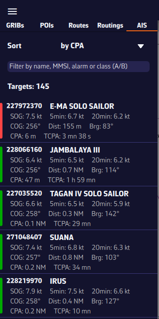
To quickly find a vessel, you can sort and filter the AIS target list.
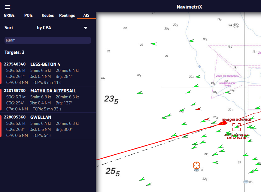
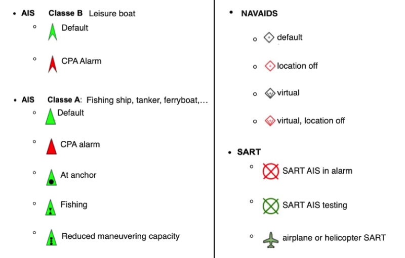
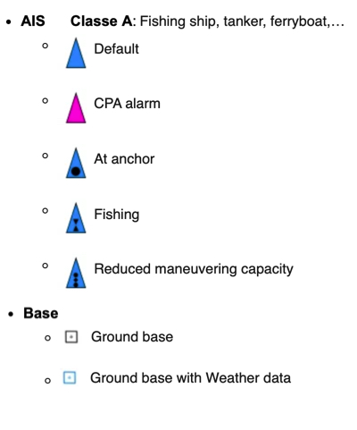
You can display several types of icons on the chart: AIS targets, navigation aids (NavAids), SART (Search And Rescue) distress beacons, AIS targets via the Internet (1st quarter of 2026), and “in-situ” weather data stations.
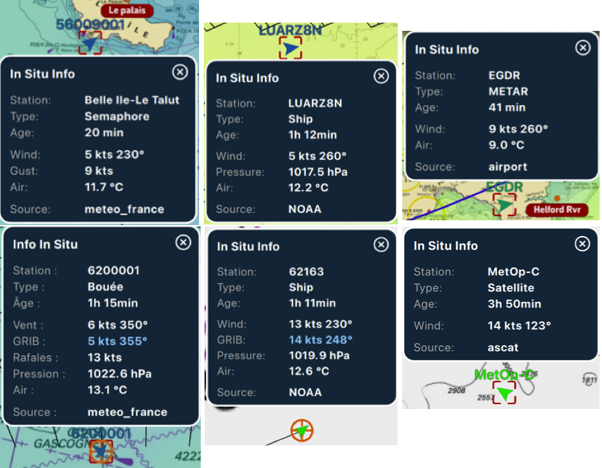
The symbol takes on the orientation and color scheme of the wind display.
If the time of the information falls within the coverage period of the GRIB file displayed, then tapping/clicking in the center of the popup centers the chart on the station’s coordinates and returns the timeline to the exact time of the station, allowing you to compare the data value and the GRIB file forecast.
NMEA activation is synchronized on all devices connected to the same Wi-Fi router (NMEA gateway, multiplexer, onboard router). Therefore, disabling NMEA on one device, such as your smartphone, disables NMEA on other devices in use, such as tablets or computers.
You have two options in the above case:
On the chart, the course vector on the ground COG is represented by a red arrow. The magnetic heading line is represented by a green line. Both are variable in length.
Open the app settings by tapping on the ⚙︎ icon, then select the My Boat section.
Open the app settings ⚙︎ and select ‘My boat’. The track settings are at the bottom of the list.
You are able to:
ZOIs are areas to avoid or areas of particular interest. Some are pre-existing in the application, but you can create as many as you need. There are three types:
Only no go zones and slow zones are considered by the routing calculation, if they are displayed on the chart. In the left side menu list, you can enable/disable the display of a zone on the chart by tap/click on the eye icon, select one or more zones to export or delete them by checking the box(es). You can also import ZOIs.
Tap/click on the border of a ZOI to edit/delete it. You can move the borders by selecting the corners, add an intermediate point anywhere on the border to modify it. After selecting the ‘Finish’ button, you can also change the name and type of the zone.
Laylines are automatically displayed when you have activated a POI using the ‘Go to’ function and you need to tack or jibe to reach your target, upwind or downwind.
By convention, the green layline is the starboard tack, and the red layline is the port tack.
You can activate the instruments corresponding to the layline data:
You can send NMEA data to instruments to:

In the Settings menu, select the GPS & NMEA option.
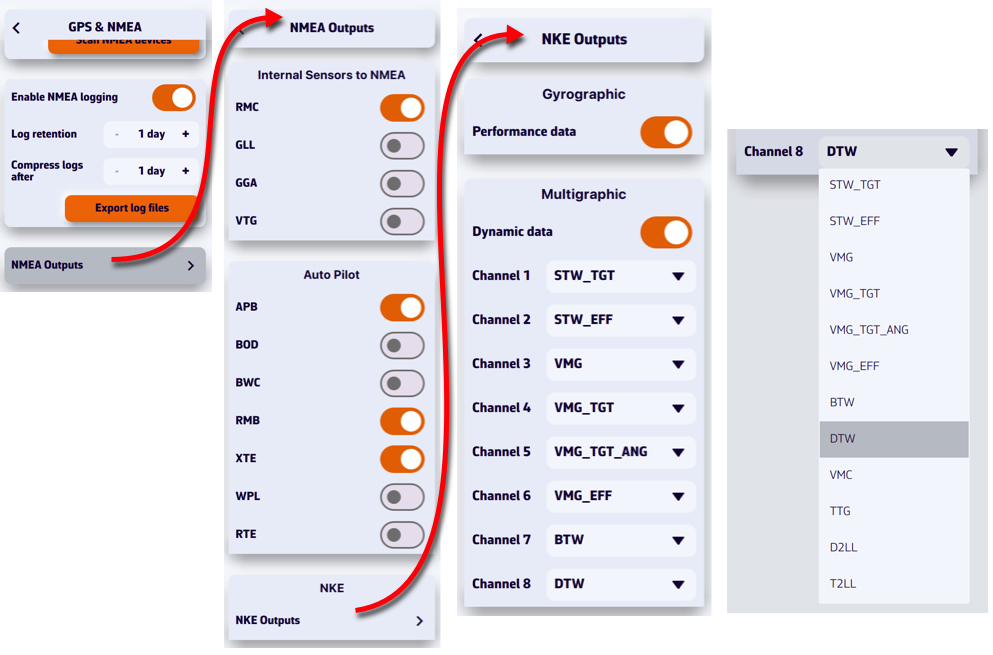
In order to be received by your instruments, the sentences must be transmitted via a bidirectional gateway or multiplexer, usually via Wi-Fi. To be processed, you must first check the sentences allowed by your instruments in their user manual (autopilot, chartplotter, repeater, etc.).
You can feed each of the 8 dynamic channels of the NKE Multigraphic from a list of sentences by scrolling down the menu for each channel.

Using the action button, you can perform several measurements on the chart. Select ‘Add a new measure’ then move the endpoints. The vector displays the distance and true bearing.
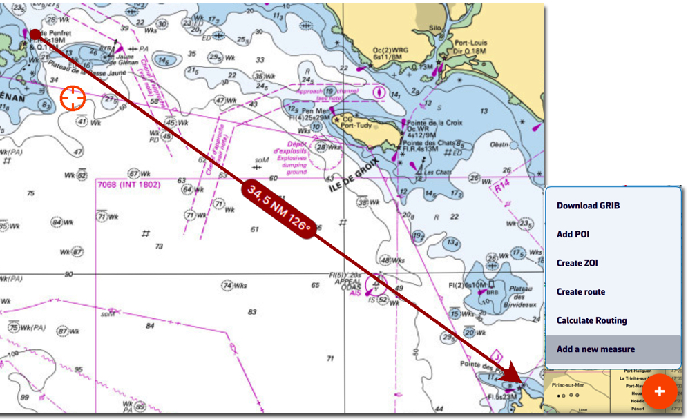
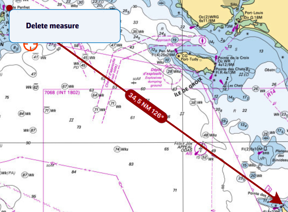
To delete the measurement, tap/click on the origin of the arrow.
From the Layers button, check the ‘Auto measure’ display option:
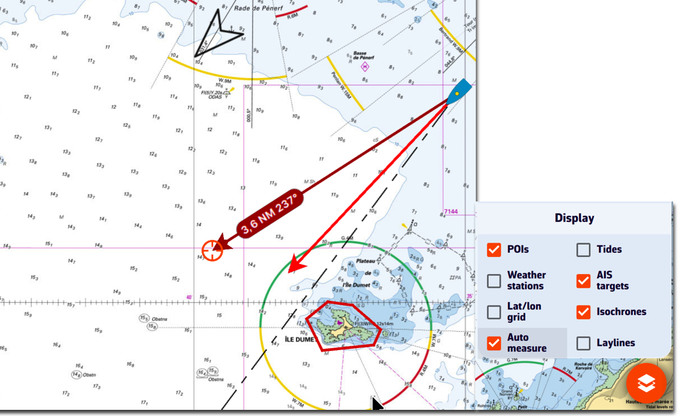
The measurement arrow is automatically displayed from your location toward the target in the centre of the screen. Simply move the chart under the target to the desired location. The distance vector is then displayed for a short time, giving you time to read the distance and true bearing. Each time the chart is moved under the target, the vector is reset.
You can disable the distance vector display by unchecking the ‘Auto measure’ box.
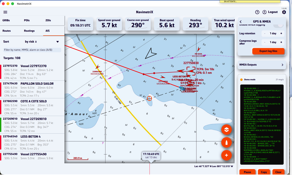
DEMO mode allows you to view a navigation routine with moving AIS targets. This gives you an idea of how the application works when you are “at home”.
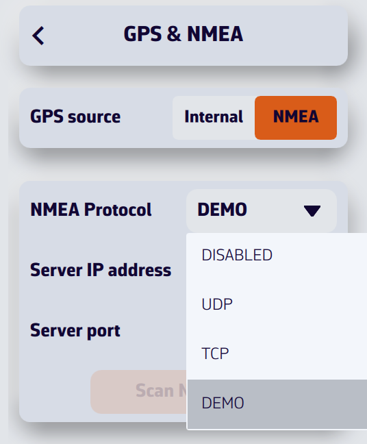
Open the settings and select the GPS & NMEA option. Select GPS source = NMEA.
In the ‘NMEA Protocol’ drop-down menu, select DEMO.
The window will then display a simulated routine allowing you to see NavimetriX in action while navigating, select AIS targets to display CPA prediction points, read target information in the side column list, view navigation data in the instruments, etc.
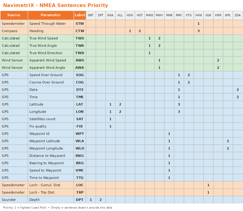
NavimetriX receives navigation data from your instruments via NMEA 0183 sentences. When multiple sentences can provide the same parameter, the app uses the highest-priority source available (1 = first choice). If that sentence isn’t received, it falls back to the next priority.
By default, the target is placed in the center of the screen, allowing you to drag the map underneath it and use the zoom to position it at a specific location.
However, you can lock the target to other elements, or even disable it.
Tap/click on the layers button.
In the “Target” drop-down menu, select which element you want to lock the target to:
You can also lock the target onto a POI by editing it.
The XDR (Transducer Measurement) sentence is a generic NMEA0183 sentence used to transmit measurements from various types of sensors (transducers). It allows multiple measurements to be grouped into a single sentence.
$xxXDR,a,x.x,u,n,a,x.x,u,n,...*hhWhere for each transducer group:
The checksum (*hh) is mandatory.
| Field | Value |
|---|---|
| Type | A (Angular) |
| Unit | D (Degrees) |
| Name | PTCH |
Example:
$IIXDR,A,5.2,D,PTCH*XXThis indicates a pitch angle of 5.2°.
| Field | Value |
|---|---|
| Type | A (Angular) |
| Unit | D (Degrees) |
| Name | ROLL |
Example:
$IIXDR,A,-1.1,D,ROLL*XXThis indicates a roll angle of -1.1°.
Combined example (Roll + Pitch):
$IIXDR,A,-1.1,D,ROLL,A,5.0,D,PTCH*74| Field | Value |
|---|---|
| Type | C (Temperature) |
| Unit | C (Celsius), F (Fahrenheit), or K (Kelvin) |
| Name | Must contain water (e.g., WATERTEMP, WaterTemp, water) |
Examples:
$IIXDR,C,18.5,C,WATERTEMP*XX
  $IIXDR,C,65.3,F,WaterTemp*XX
$IIXDR,C,291.65,K,water*XX| Field | Value |
|---|---|
| Type | C (Temperature) |
| Unit | C (Celsius), F (Fahrenheit), or K (Kelvin) |
| Name | Must contain air (e.g., AIRTEMP, AirTemp, air) |
Examples:
$IIXDR,C,22.0,C,AIRTEMP*XX
  $IIXDR,C,71.6,F,AirTemp*XX
Combined example (Water + Air):
$IIXDR,C,18.1,C,WATERTEMP,C,22.0,C,AIRTEMP*49| Field | Value |
|---|---|
| Type | P (Pressure) |
| Unit | B (Bars) |
| Name | Must contain baro (e.g., BARO, Barometer, baro) |
Note: The value must be expressed in Bars (1 bar = 1000 hPa). NavimetriX automatically converts it to hPa.
Example:
$IIXDR,P,1.013,B,BARO*XXThis indicates a pressure of 1013 hPa.
Transducer groups can be chained in the same XDR sentence (up to 10 transducers per sentence):
$IIXDR,A,-2.5,D,ROLL,A,3.1,D,PTCH,C,18.5,C,WATERTEMP,C,21.0,C,AIRTEMP,P,1.015,B,BARO*XXNo. Transducer name recognition is not case-sensitive for temperatures and pressure:
WATERTEMP, WaterTemp, watertemp → all recognizedAIRTEMP, AirTemp, airtemp → all recognizedBARO, Barometer, baro → all recognizedException: For roll and pitch, the names must be exactly ROLL and PTCH.
NavimetriX accepts all standard talker prefixes (II, GP, HC, etc.). The examples above use $II (Integrated Instrumentation), but $GP, $HC, or others are equally valid.
| Measurement | Type | Unit | Transducer Name |
|---|---|---|---|
| Pitch | A | D | PTCH |
| Roll | A | D | ROLL |
| Water temperature | C | C, F, or K | contains water |
| Air temperature | C | C, F, or K | contains air |
| Barometric pressure | P | B | contains baro |
The NavimetriX interface has been designed to be clear, intuitive, and quick to use, whether on a computer, tablet, or smartphone. Here is a complete description, section by section:
☰ Hamburger menu: provides access to the application’s main lists:
In order for NavimetriX to be synchronised across two or more devices, you must:
Most settings are synchronised, with a few exceptions, namely:
Downloaded GRIB files appear in the GRIB list on all devices. When a GRIB is downloaded or updated on a device, it is followed by a dimmed refresh icon. If a new run is available for that GRIB, this icon is activated.
On other device(s), the list of downloaded GRIBs is displayed but followed by an activated download icon. The contents of the GRIBs must then be downloaded manually.
The Geogarage account is synchronised across all devices.
Geogarage charting is not synchronised: charts must be downloaded to each device.
You will find a short tutorial on the basic functions of NavimetriX by following Get Started.
Before writing to us, please check the FAQs — you’ll probably find the answer to your question 😉.
There’s no need to browse through all the FAQs one by one: you can search within the FAQs, so don’t hesitate to use the search bar!
📘 This glossary brings together the main terms used in the Navimetrix application and its FAQs. It helps users better understand concepts related to navigation, routing, and marine weather.
The actual direction of the boat’s movement over the seabed, expressed in degrees relative to true north. It differs from the compass heading when there is drift caused by wind or current.
The boat’s actual speed relative to the ground (not the water). Calculated by GPS, it includes the effect of currents.
The direction in which the boat’s bow is pointing, measured relative to true or magnetic north.
The angle between the boat’s axis and the true wind direction. It is calculated from the apparent wind and the boat’s speed.
The wind speed derived from the apparent wind and the boat’s speed. It represents the actual wind strength on the sea surface.
The wind angle felt on board, influenced by the boat’s motion. Measured relative to the boat’s centerline.
The wind speed felt on the boat, resulting from the combination of the true wind and the boat’s speed.
The useful component of the boat’s speed, indicating the effective progress toward the destination or upwind.
The point at which two vessels will be at their minimum distance from each other, based on their current courses and speeds.
The time remaining before reaching the CPA, used for collision avoidance and AIS alarms.
The angle between north and the direction of an observed object from the boat. Used to determine the relative position of a target or coastline.
The water depth below the keel, measured by an echo sounder. A key parameter for safe navigation.
A geographic point used to define a route or a key position. In Navimetrix, POIs represent these waypoints.
A standard file format containing numerical weather forecasts (wind, waves, pressure, temperature, etc.).
A curve connecting all possible boat positions at a given time according to the predicted weather conditions.
The calculation of an optimal route considering wind, waves, currents, and the boat’s performance.
A performance curve showing the boat’s speed as a function of wind angle and wind strength. It forms the basis for the routing engine.
The predicted time of arrival at the destination, calculated from the remaining distance and the average speed.
A description of the waves and swell (height, direction, period). Used to assess routing comfort and safety.
A regular train of waves formed by distant winds. It differs from the wind sea, which is generated locally.
The average height of the highest one-third of waves, the main indicator of overall sea conditions.
Water movements caused by tides or ocean circulation. They affect the boat’s speed and trajectory.
Variation in sea level caused by the gravitational attraction of the Moon and the Sun. It influences depth and coastal currents.
These operating system versions are prerequisites for running NavimetriX, as they define compatibility with our development framework.
However, they do not guarantee that the application will be fully compatible with your device. Other factors such as insufficient RAM or a low-performance graphics processor may also affect performance and compatibility.
⚠️ If you receive a warning from your antivirus, it is most likely a false positive.
You can check on VirusTotal that our .exe file is clean and recognized as safe by major antivirus programs.
Resolving an issue on a Windows PC can be complex, given the wide variety of possible configurations. Here are some basic steps to check:
If these steps do not solve the problem, your PC may not be compatible due to insufficient RAM or a graphics card that does not meet the app’s requirements.
To uninstall the application:
The application will be uninstalled, and all folders where it stores data as well as its registry keys will be removed.
You can also use the CleanMyMac application.
In the Settings panel, the first section covers the basic configuration options:
With a Premium subscription, you’ll enjoy the full potential of the application.
In addition to all the features of the free version:
You’ll benefit from a 7-day free trial period, so don’t hesitate to give it a try — we’re confident you’ll be convinced.
The Premium subscription is annual and renews automatically.
The price depends on the region where you subscribe.
For example, it is:
Please note that the subscription does not include nautical charts. To navigate with marine charts, you need to have a subscription on the Geogarage platform.
At the moment, you cannot subscribe directly from a Windows PC. To get a subscription, please use your phone (or tablet) via the App Store for iOS or macOS, or the Play Store for Android.
This subscription will then be valid on all your devices, including your PC.
When renewing a subscription or at the end of the trial period, in order to update our database with the information provided by the App Store, you must launch the application on the device that took out the subscription.
Important: On your PC or any device where you did not take your subscription, make sure to login to your NavimetriX account to see your subscription
Cancellation is done through your Apple account.
To turn off an automatically renewing subscription on an Apple device (iOS/iPadOS):
Settings > Your Account > Subscriptions > Select the subscription > Cancel Subscription
To cancel a subscription on a Mac, follow this link.
Note: Do not cancel before the end of the 7-day free trial if you wish to keep Premium access. However, if you do not want to subscribe, you must cancel before the end of the 7th day to avoid being charged.
Cancellation is done through your Play Store account.
To turn off an automatically renewing subscription on an Android device:
Follow the instructions on this page.
Note: Do not cancel before the end of the 7-day free trial if you wish to keep Premium access. However, if you do not want to subscribe, you must cancel before the end of the 7th day to avoid being charged.
The NavimetriX interface has been designed to be clear, intuitive, and quick to use, whether on a computer, tablet, or smartphone. Here is a complete description, section by section:
☰ Hamburger menu: provides access to the application’s main lists:
In order for NavimetriX to be synchronised across two or more devices, you must:
Most settings are synchronised, with a few exceptions, namely:
Downloaded GRIB files appear in the GRIB list on all devices. When a GRIB is downloaded or updated on a device, it is followed by a dimmed refresh icon. If a new run is available for that GRIB, this icon is activated.
On other device(s), the list of downloaded GRIBs is displayed but followed by an activated download icon. The contents of the GRIBs must then be downloaded manually.
The Geogarage account is synchronised across all devices.
Geogarage charting is not synchronised: charts must be downloaded to each device.
In the Settings panel, the first section covers the basic configuration options:
Some settings are essential — both for safety and for the proper functioning of the application.
You and your crew members must be able to access the navigation app instantly, whatever the situation. At sea, a code is useless — even dangerous if you are unable to handle navigation yourself: your crew must be able to take over quickly.
Unexpected sleep mode during a critical navigation moment (e.g., nighttime landfall in the rain in an unknown area) can be dangerous if you cannot instantly relaunch the app (e.g., wet fingers or touchscreen not responding). You should manually activate or deactivate your device depending on the situation.
In addition, sleep mode interrupts track recording.
This prevents wasting time when entering text in the app, such as route names, POIs, etc.
Regarding onboard computers, PC or Mac, the same recommendations apply. Adjust the settings according to the operating system and version used.
This setting allows you to enlarge or reduce the size of all elements displayed on the map (up to 140%, for example). Very useful on board if you want to use the app without wearing your glasses.
Note that the menu font size remains unchanged.
Your boat’s polar determines all routing calculations. It represents your boat’s performance depending on wind speed and angle.
The application supports files in the .pol format (also used by Weather4D, SailGrib, Adrena, and others).
To choose your boat’s polar from the library:
Most of these polars come from naval architects or ORC certificates.
To find your polar, you can:
Once you’ve found your polar, select it and it will be confirmed.
Comment importer une polaire?
The application can import polars in the .pol format.
To import your own polar:
iPolar lets you create a polar in one minute based on your boat’s characteristics:
Note: The iPolar method was developed by KND, experts who work with the America’s Cup, TP52s, and IMOCAs — the best in their field!
Some polars are formatted as .CSV (Comma Separated Value) files, where the field separator is a comma or semicolon. This format is not supported in NavimetriX, unlike the .POL format where fields are separated by tabs — a format widely used in navigation applications. Therefore, you need to convert your .CSV file to .POL.
Open a new Excel sheet and select the menu: File > Import.
Choose “CSV File” and then select your polar file from the Finder.
Check the box Delimiters = “Semicolon”, then insert the data into the existing sheet.
Then save the file in “Text (Tab delimited)” format, which will create a .TXT text file.
Finally, rename the file by replacing the .TXT extension with .POL:
Your polar file is now ready to be imported.
Open the .CSV file with Numbers:
Export the file to TSV:
Replace the file .TSV extension to .POL, that’s all.
On the chart, the course vector on the ground COG is represented by a red arrow. The magnetic heading line is represented by a green line. Both are variable in length.
Open the app settings by tapping on the ⚙︎ icon, then select the My Boat section.
Open the app settings ⚙︎ and select ‘My boat’. The track settings are at the bottom of the list.
You are able to:
Procedure:
NavimetriX.exe file in its installation folder).By default, the target is placed in the center of the screen, allowing you to drag the map underneath it and use the zoom to position it at a specific location.
However, you can lock the target to other elements, or even disable it.
Tap/click on the layers button.
In the “Target” drop-down menu, select which element you want to lock the target to:
You can also lock the target onto a POI by editing it.
A GRIB file (for GRIdded Binary) is a standard file format used by meteorological services to distribute numerical weather forecasts.
It contains the raw data generated by weather models (wind, pressure, rain, waves, currents, etc.) organized on a grid covering a geographic area.
Why use this format?
What does a GRIB file contain?
Depending on the selected model, a GRIB file may include:
What is it used for in navigation?
A GRIB file allows you to visualize the evolution of the weather over a given area directly within your navigation software or weather app.
To illustrate the process, let’s say we’re planning a 4-day passage from La Rochelle (France) to Cowes (UK).
A Download GRIB window opens. The choices are filtered to your selected region.
Without the Premium option, you’re limited to the GFS model (the U.S. NOAA global atmospheric model).
The estimated compressed GRIB size appears at the bottom. Keep it reasonable—if you see ~200 MB, you probably chose a model that’s too fine or too many parameters.
Below the model description, we show the latest model calculation time (the Run).Run: 20251016 12Z +102 means: calculated on Oct 16, 2025; initialized at 12:00 UTC (12Z); contains 102 forecast hours from that run.
We also display the estimated time until the next run is available.
You may have noticed a small icon on the right of each item in the GRIB files list. This icon shows the update status of your GRIB file and can display three different states:
The icon appears in dark orange right after a GRIB file has been downloaded. This means your file is up to date — you already have the latest available version of the weather model.
This is what you will see immediately after downloading a GRIB file.
The icon turns light orange. This means a new model run (a new forecast) is available. To update your GRIB file, simply click or tap on this icon: the file will automatically be replaced with the latest version.
Finally, the icon may appear in light orange with a small download symbol. This means you have already downloaded this GRIB file on another device, but it is not yet available locally on the one you are using. To retrieve it, simply click or tap on the icon: the file will be downloaded automatically.
Global models (such as GFS or ECMWF) cover the entire planet. They are essential for long crossings and long-term forecasts (up to 10–15 days), but their resolution remains limited (20 to 50 km). They are used to get an overall view of the weather and for long-distance passages.
Regional models focus on a specific area (France, Europe, the Mediterranean…). Their coverage is smaller, but their resolution is much finer (2 to 10 km), allowing for better anticipation of local effects such as thermal breezes, thunderstorms, terrain, and coastal winds. In return, they generally only extend 2 to 3 days into the future. They are used for day trips or short cruises.
If you’re not familiar with weather models, you’re probably wondering which ones to choose.
Here are a few simple rules:
Select the model according to your navigation area and type of sailing, following the table below.
For weather data, if in doubt, choose the ECMWF IFS model.
The ECMWF IFS model covers the entire globe for up to 14 days. However, note that forecast reliability decreases with time:
| Forecast range | Reliability level |
|---|---|
| Up to 2 days | Excellent |
| 2–4 days | Very good |
| 4–5 days | Good |
| 5–8 days | Reasonable trend |
| 8–10 days | Rough trend |
| Beyond | At best a trend — often unreliable. Prefer the AIFS model, computed using Artificial Intelligence. |
Here’s a table to help you choose. We’ll soon add an automatic selection feature based on your sailing program.
| Type of data | Type of navigation | France – Atlantic & Channel | France – Mediterranean | Europe (outside France) | United States | Rest of the World |
|---|---|---|---|---|---|---|
| Weather | Day sailing in a bay | Arome | Arome | UKV, ICON, or Arpege Europe | Nam Conus Nest | ECMWF IFS |
| Weather | Coastal | Arpege Europe | Arpege Europe | UKV, ICON, or Arpege Europe | Nam Conus | ECMWF IFS |
| Weather | Offshore | ECMWF IFS and AIFS + GFS | ECMWF IFS and AIFS GFS | ECMWF IFS and AIFS GFS | ECMWF IFS and AIFS GFS | ECMWF IFS and AIFS GFS |
| Waves | Coastal | MFWAM France | MFWAM France | MFWAM | GFS Wave | GFS Wave |
| Waves | Offshore | MFWAM + GFS Wave | MFWAM + GFS Wave | MFWAM + GFS Wave | MFWAM + GFS Wave | MFWAM + GFS Wave |
| Currents | Day sailing in a bay | Ifremer | Copernicus Med | Copernicus | MSC NCOM | Copernicus SMOC |
| Tidal currents | Coastal | Copernicus IBI | Copernicus Med | Copernicus IBI or ENWS | MSC NCOM | Copernicus SMOC |
| Ocean currents | All | Copernicus IBI | Copernicus Med | Copernicus IBI or ENWS | Copernicus Global | Copernicus Global |
These models provide a simplified description of the sea state.
In short, they include the significant height of the total sea, its period, its direction, as well as the same information for the wind sea.
They are mainly used in routing when conditions are challenging.
See also: It’s great to have all these models — but which one should I choose?
Open the Settings panel by tapping the cogwheel at the top right of the upper ribbon, then select GRIB Display.
In the “Wind” section, select Particles or Barbs. Animated particles show the wind flow but consume more system resources and therefore battery — best avoided while sailing. Vectors and barbs are the classic meteorological representation of wind direction and strength. They are positioned on each grid point of the GRIB file and are more resource-efficient.
The Gradient style represents wind strength using a rainbow color scale — from blue (light or calm winds) to magenta (strong winds), through shades of green, yellow, orange, and red. Especially suitable for wind data.
The Isoplane style displays the data with the same colors but as equal-value zones. This style is better suited for data such as wave height, for example in 50-cm increments.
The Land Mask displays data over land as well. This is particularly useful when sailing among islands, to keep a continuous sea/land display.
Transparency allows you to adjust the color overlay depending on the background (satellite map or nautical chart).
The Iso-zone step adjusts the spacing between isoplane zones depending on the type of data (waves, precipitation, temperature, etc.).
On the map, the Layer button at the bottom right of the screen lets you choose what to display.
In the GRIB Display section, the drop-down menu allows you to select which data to display. If a weather GRIB (for example an IFS model) is displayed, Wind will be selected by default. You can enable or disable the color background, particles or barbs (according to your previous setting above), and isobars (lines of equal atmospheric pressure).
If you have displayed a wave GRIB file, you can enable or disable the color background and the wave direction arrows.
This section automatically adapts to the type of GRIB file displayed on the screen: weather, waves, or currents.
By default, a tide gauge is displayed on the cartography for each referenced station.
The display can be disabled by opening the layers menu and unchecking the Tide box. The gauges currently display dynamically:
Tapping on each gauge opens a tide graph showing the tide curve and the current water level, represented by the vertical timeline.
The graph is topped by a table showing the times, water heights and tidal coefficients for the day.
Tapping/clicking on the date above the table opens the calendar, allowing you to select another day/month.
The height threshold can be used to determine:
NavimetriX offers several high-resolution regional models for popular sailing destinations worldwide, in addition to global models like GFS, ECMWF, and ICON Global.
NAM (11 km resolution) — NOAA’s North American Mesoscale model covers the continental United States. Forecasts up to 84 hours with hourly time steps. Ideal for coastal navigation along the US East Coast, West Coast, and Gulf of Mexico.
HRRR CONUS (3 km resolution) — The High-Resolution Rapid Refresh model provides the finest resolution for the continental US. Forecasts up to 18 hours, updated hourly. Perfect for racing and detecting rapidly evolving conditions like sea breezes and thunderstorms.
Arome Antilles (3 km resolution) — Météo-France model covering the Lesser Antilles from Puerto Rico to Trinidad. Forecasts up to 48 hours. Excellent for inter-island passages and detecting trade wind variations.
Arome Guyane (3 km resolution) — Covers waters off French Guiana and the nearby South American coast. Forecasts up to 33 hours. Useful for sailors transiting between the Caribbean and Brazil.
Arome Polynésie (3 km resolution) — Covers French Polynesia including Tahiti and the Society Islands. Forecasts up to 48 hours. Ideal for detecting local effects around high volcanic islands and reef passes.
Arome Calédonie (3 km resolution) — Covers New Caledonia and the Coral Sea. Forecasts up to 48 hours. Essential for navigating the lagoon system and anticipating thermal effects around Grande Terre.
Arome Réunion-Mayotte (3 km resolution) — Covers the western Indian Ocean from the Mozambique Channel to the Mascarene Islands, including Madagascar, Réunion, Mauritius, and Mayotte. Forecasts up to 48 hours. Critical for this cyclone-prone region.
NavimetriX provides access to over 70 weather, wave, and current models from leading meteorological agencies worldwide.
GFS — NOAA — 28 to 222 km — 16 days
ECMWF IFS — ECMWF — 28 to 111 km — 15 days
ECMWF AIFS — ECMWF — 28 to 111 km — 15 days
ICON Global — DWD — 14 to 111 km — 5 days
Arpège Monde — Météo-France — 28 km — 4 days
GDPS (GEM) — CMC Canada — 17 km — 10 days
Arpège Europe — Météo-France — 11 km — 4 days
Arome — Météo-France — 3 km — 42 hrs
Arome HD — Météo-France — 1 km — 36 hrs
ICON Europe — DWD — 8 km — 5 days
ICON D2 — DWD — 2 km — 48 hrs
UKV — Met Office — 6 km — 5 days
NAM — NOAA — 11 km — 84 hrs
HRRR CONUS — NOAA — 3 km — 18 hrs
Arome Antilles — Météo-France — 3 km — 48 hrs
Arome Guyane — Météo-France — 3 km — 33 hrs
Arome Polynésie — Météo-France — 3 km — 48 hrs
Arome Calédonie — Météo-France — 3 km — 48 hrs
Arome Réunion-Mayotte — Météo-France — 3 km — 48 hrs
GFS Wave — NOAA — Global — 28 to 111 km — 16 days
MFWAM Global — Météo-France — Global — 11 to 56 km — 4 days
MFWAM France — Météo-France — France — 3 km — 4 days
IFREMER WW3 — Ifremer — France coasts (14 zones) — 190m to 500m — 4 days
Copernicus Global — Copernicus — 9 km — 5 days — oceanic currents only (Gulf Stream, etc.)
Copernicus Global SMOC — Copernicus — 9 to 56 km — 5 days
Copernicus IBI — Iberian-Biscay-Ireland — 3 km — 5 days
Copernicus ENWS — NW Shelf / North Sea — 2 km — 5 days
Copernicus BALTIC — Baltic Sea — 4 km — 5 days
Copernicus MED — Mediterranean — 5 km — 5 days
SHOM Manche-Gascogne — Channel & Biscay — 2 km — 5 days
SHOM Méditerranée Nord — NW Mediterranean — 2 km — 5 days
IFREMER — France coasts (10 zones) — 250m to 3 km — 4 days
MSC Saint Laurent — St. Lawrence / Atlantic Canada — 1 km — 84 hrs
NCOM Alaska – N. Calif — Alaska to N. California — 4 km — 90 hrs
NCOM Caribbean — Gulf of Mexico & Caribbean — 3 km — 90 hrs
NCOM Hawaii — Hawaii — 4 km — 90 hrs
NCOM South California — Southern California — 4 km — 90 hrs
NCOM US East Coast — US East Coast — 4 km — 90 hrs
In order to rename a GRIB file, you must click/press and hold on its name. This will bring up the keyboard, allowing you to change the name:
The name will be preserved during updates and synchronization.
The term “waypoint” doesn’t exist in NavimetriX. Instead, we use POI (Point Of Interest), a more generic term that can include many elements (targets, anchorages, beacons, race marks, etc.).
Drag the map under the target on the screen, zooming in to position it accurately.
Tap the + icon in the bottom right corner of the screen and select ‘Add POI’ from the menu.
Tap OK to confirm.
Place the mouse or trackpad pointer on the desired location on the map, without worrying about the target, and right-click. In the popup that appears, select “Add a POI”. The creation window opens as shown here.
Alternatively, you can proceed the same way as on a tablet or smartphone.
The points are saved in the POI list, located in the left sidebar of the screen, accessible via the ≡ symbol in the top-left toolbar.
You can show or hide each point individually by tapping the eye icon on the right side of the column.
You can adjust the display so that the name and optional icon appear only from a certain zoom level, preventing the map from becoming overloaded if you have many points.
Move the chart under the target displayed on the screen, zooming in for precise positioning, then tap the + icon in the lower right corner. From the menu, select “Create a route”.
Tap successively to place the desired points. You can drag them with your finger to move them if needed. Zoom in for more precise placement. Once finished, select the “Finish” button at the top of the screen. Enter a name for your route and confirm saving by tapping “OK”.
Click to create successive points, zooming in for better accuracy. You can also drag the points to adjust their position if needed. Click the “Finish” button at the top of the screen. Enter a name for your route and confirm saving by clicking “OK”. Alternatively, you can proceed the same way as on a tablet or smartphone.
In any case, you can also create a route by tapping or clicking an existing POI (waypoint) and selecting “Begin route” from the popup menu starting from that point.
Routes are saved in the Routes list, located in the left sidebar of the screen, accessible via the ≡ symbol in the top-left toolbar.
Tap the “eye” icon next to each route to toggle its display on or off. Use the checkboxes to select routes for export or remove.
A “Table” icon allows you to open the detailed route info. Tap/clic “Reverse route” button to sail back.
Tap or click, depending on your device, on a POI, and in the menu that appears select “Edit POI” to open the edit window.
See also: How do I create a POI or waypoint
Open the left sidebar and select the “Routes” section. Display the route on the map by activating the “eye” symbol, then tap or right-click (depending on your device) on any part of the route. In the menu that appears, choose the option “Edit route”.
You can then drag points on the map to move them, add new ones by tapping on a segment of the route, and edit or delete any existing route point.
See also: How do I create a route?
To start navigation toward a POI (or Waypoint):
💻 On a computer: right-click the waypoint you previously saved, then select Go to. Confirm that you want to navigate to this waypoint.
📱 On a mobile device or tablet: tap the POI, then select Go to and confirm navigation.
Once the POI is selected, if the boat (the GPS) is at sea, a black dashed line is drawn between your boat and the POI.
To stop navigation, tap or click again on the POI you are navigating to, then choose Stop goto from the menu.
Your boat’s polar determines all routing calculations. It represents your boat’s performance depending on wind speed and angle.
The application supports files in the .pol format (also used by Weather4D, SailGrib, Adrena, and others).
To choose your boat’s polar from the library:
Most of these polars come from naval architects or ORC certificates.
To find your polar, you can:
Once you’ve found your polar, select it and it will be confirmed.
Comment importer une polaire?
The application can import polars in the .pol format.
To import your own polar:
iPolar lets you create a polar in one minute based on your boat’s characteristics:
Note: The iPolar method was developed by KND, experts who work with the America’s Cup, TP52s, and IMOCAs — the best in their field!
Some polars are formatted as .CSV (Comma Separated Value) files, where the field separator is a comma or semicolon. This format is not supported in NavimetriX, unlike the .POL format where fields are separated by tabs — a format widely used in navigation applications. Therefore, you need to convert your .CSV file to .POL.
Open a new Excel sheet and select the menu: File > Import.
Choose “CSV File” and then select your polar file from the Finder.
Check the box Delimiters = “Semicolon”, then insert the data into the existing sheet.
Then save the file in “Text (Tab delimited)” format, which will create a .TXT text file.
Finally, rename the file by replacing the .TXT extension with .POL:
Your polar file is now ready to be imported.
Open the .CSV file with Numbers:
Export the file to TSV:
Replace the file .TSV extension to .POL, that’s all.
To compute a routing, you must first have:
Once these 3 steps are done, you can compute a routing by pressing the “Compute routing” button.
Remember: a routing is only useful if it’s correctly calibrated and you understand the computed result. Doing a single run and treating it like a train timetable will, at best, lead to disappointment.
We therefore recommend this approach:
Click the “+” button, then select “Compute a routing”. A screen titled Routing opens.
You can choose three forecast models:
To begin, select only a wind forecast file.
We recommend setting the wind factor to 115%. This means taking 115% of the wind speed from the GRIB, reflecting that GRIB wind speeds are often lower than reality.
In a second step, following our recommendations, select a current model and a wave model.
Click the date to open the calendar and select your departure date. Click OK.
Click the time to open hour/minute selection, then also validate with OK.
Select the route you just created.
These are less frequently modified, but here are the main parameters at a glance.
Useful for studying, for example, the effect of current in a bay. It freezes the wind (e.g., as measured at the masthead) to understand the current’s influence on the optimal route.
Allows you to constrain the optimal route. Use with care, otherwise the routing may not converge. For example, don’t set a max downwind wind speed of 20 kn for an ocean passage.
We define a cross sea when the angle between total sea direction and wind sea direction is between 45° and 135°. If the total sea height is high enough, the boat is significantly slowed. You can set the slowdown parameters here.
It’s easy to get a bit lost among all these settings. The default values were chosen carefully. Press this button to restore them.
Once the routing is computed, the optimal route is shown on the chart together with the isochrone curves. These curves represent the positions that can be reached at successive time intervals from the start point.
You can move the boat along the route in two ways:
At each intersection between the optimal route and an isochrone, a wind barb is drawn. It shows the wind speed and direction at the time the boat reaches that position. If you route with current, a current arrow will also be drawn
Open the lists panel (via the ☰ button at the top left of the screen) and select the Routing tab. This tab lists all computed routings.
For each routing you’ll see:
Click the orange button to open the routing table. It contains four tabs, each presenting a different facet of the computation.
A pivot point is a location you want the routing to pass through.
It’s a very useful way to quickly compare routing options.
For example, in this case we’ll check whether it’s better to pass inside or outside the Traffic Separation Scheme (TSS) off Cape Finisterre — a very common situation when sailing from the French Atlantic coast toward Madeira or the Canary Islands.
To perform a routing with a pivot point, first make sure the isochrones of the desired routing are displayed on the map.
First you have to verify that Isochrones are checked in the Display section of layers menu:
Then simply tap/click on the name of the routing in the sidebar:
When isochrones are displayed, you can use a pivot point.
ZOIs are areas to avoid or areas of particular interest. Some are pre-existing in the application, but you can create as many as you need. There are three types:
Only no go zones and slow zones are considered by the routing calculation, if they are displayed on the chart. In the left side menu list, you can enable/disable the display of a zone on the chart by tap/click on the eye icon, select one or more zones to export or delete them by checking the box(es). You can also import ZOIs.
Tap/click on the border of a ZOI to edit/delete it. You can move the borders by selecting the corners, add an intermediate point anywhere on the border to modify it. After selecting the ‘Finish’ button, you can also change the name and type of the zone.
When isochrones are displayed, data labels in the same colour as the routing boat allow you to track progress along the route. In addition, clicking/tapping on each label displays the data graph from the start to the end of the route.
To scroll the boat along the route, a weather model must be displayed to activate the timeline.
A routing table is generated automatically and appears as an icon next to the route. Simply tap/click on the icon to display it.
Today, marine charting compatible with the app is provided exclusively by the Geogarage platform, where you must create an account and subscribe to one or more chart services depending on your sailing areas.
The charts available come from the official digital data of many international hydrographic offices such as the SHOM, UKHO, NOAA, and others.
Currently, about thirty publishers are available, offering near-global coverage. These are raster charts divided into tiles, allowing smooth zooming between scales.
When you subscribe to a hydrographic service via Geogarage, you gain access to all the charts published by that hydrographic office.
For example, if you subscribe to the SHOM (Service Hydrographique et Océanographique de la Marine) charts, you will have access to all SHOM charts.
Thus, if you’re sailing from La Rochelle to Fort-de-France across the Atlantic, a single SHOM chart subscription is probably sufficient to cover your entire passage.
As a reference:
Below is an illustration showing the diversity of hydrographic services available through Geogarage:
Select a hydrographic service to view the chart coverage included with that subscription.
Annual subscription prices (VAT included)
In the Settings of Navimetrix, under the Geogarage Charts menu, you need to log in by tapping the “Login” button and entering your Geogarage account credentials.
Once connected, select your subscribed chart service (for example UKHO) from the “Layer” dropdown list. The chart display updates instantly while connected to the internet.
In the Settings of NavimetriX, under the Geogarage Charts section, tap “Add New Zone”, then define the geographical area to download by dragging the green corners of the grey rectangle.
The Area selection dropdown menu offers two zoom-level options for the maximum chart scale:
Once confirmed, a countdown shows the preparation and download progress.
A green frame remains visible so you can add new adjacent download zones without overlap using the “Add a new area” button. Only downloaded charts are available for offline use.
The downloaded chart zones are listed by publisher in the Geogarage Charts drawer. A checkbox allows you to select them for the Delete or Refresh functions.
Whenever a chart update is published by the provider, the Refresh button next to each zone becomes active. You can update them individually or in bulk by checking multiple boxes and pressing “Refresh Selected”.
In order to rename a chart area, you must click/press and hold on its name. This will bring up the keyboard, allowing you to change the name:
The name will be kept during updates and synchronization.
While sailing, if you want to display your phone’s GPS data, open the app settings (gear icon in the top-right corner).
Go to the GPS & NMEA menu and make sure the GPS source is set to Internal.
Exit this menu, then open Instruments. Check the Visible box to show the instruments, and make sure the selected layout is GPS View.
Once your phone receives a GPS signal, the time of the last position, your speed over ground (SOG), and your course over ground (COG) will be displayed in the instrument bar.
You can scroll through the parameters to view your coordinates and POI data if you’ve selected a waypoint using the Go to function.
On phones, the default display is horizontal.
On tablets or computers, the layout automatically adjusts to a vertical view.
To activate navigation toward a POI (or Waypoint):
💻 On a computer: right-click the waypoint you previously saved, then select the Go to option. Confirm that you want to navigate to this waypoint.
📱 On mobile or tablet: tap the POI, then select Go to and confirm the navigation.
Once the POI is selected, a dashed black line is drawn between your boat and the POI, showing the direct route.
To stop navigation, select the same POI again, then choose Stop Goto from the menu.
Not yet. USB GPS receivers are not currently supported directly by the application.
For now, only GPS devices transmitting NMEA data over Wi-Fi are compatible.
To change the displayed instruments, open the right panel using the gear button at the top right of the screen, then select Instruments.
You will see several settings:
On a computer, right-click an instrument. On a mobile device, perform a long tap.
A list of parameters appears — select the one you want to assign to that instrument.
To save a configuration, press the Save Configuration button, enter a name, and confirm to save it.
Saved configurations are specific to each device — they are not synchronized between your phone and your computer, ensuring optimized layouts for each screen.
To receive NMEA data from your onboard instruments:
The first line corresponds to the GPS source. If you want to receive GPS data through an NMEA stream, select NMEA.
If you don’t know these values, press Scan for NMEA Streams. The scan will automatically search for known configurations. When a stream is detected, NavimetriX will offer to apply the parameters automatically (protocol, IP, port). Select Yes and close the scanner — your NMEA source is now active!
Once connected, NMEA data appears in green in the log window at the bottom of the panel.
If no stream is found, enter your NMEA system parameters manually. We recommend using the UDP protocol for maximum flexibility.
The last section lets you enable NMEA logging. When enabled, all received NMEA sentences are recorded. You can set a retention period (for example, 8 days) and specify when the logs should be compressed. Uncompressed daily files can be large (around 60 MB), but once compressed, they are only about 10% of their original size.
The Export Logs button allows you to save these files for analysis or replay with external tools such as VDR Player.
Note: A built-in feature to replay NMEA logs will be added in a future version of the app.
Prerequisite: make sure your NMEA stream is properly configured and that you are receiving AIS sentences (they start with AIVDM).
You can hide Class B AIS targets (small recreational boats) to show only Class A (cargo, ferries, etc.)—useful at crowded race starts.
Open the hamburger menu (☰ top left) and choose the AIS tab to display the target list.
For each AIS vessel, the following information is available:
To quickly find a vessel, you can sort and filter the AIS target list.
You can display several types of icons on the chart: AIS targets, navigation aids (NavAids), SART (Search And Rescue) distress beacons, AIS targets via the Internet (1st quarter of 2026), and “in-situ” weather data stations.
The symbol takes on the orientation and color scheme of the wind display.
If the time of the information falls within the coverage period of the GRIB file displayed, then tapping/clicking in the center of the popup centers the chart on the station’s coordinates and returns the timeline to the exact time of the station, allowing you to compare the data value and the GRIB file forecast.
NMEA activation is synchronized on all devices connected to the same Wi-Fi router (NMEA gateway, multiplexer, onboard router). Therefore, disabling NMEA on one device, such as your smartphone, disables NMEA on other devices in use, such as tablets or computers.
You have two options in the above case:
On the chart, the course vector on the ground COG is represented by a red arrow. The magnetic heading line is represented by a green line. Both are variable in length.
Open the app settings by tapping on the ⚙︎ icon, then select the My Boat section.
Open the app settings ⚙︎ and select ‘My boat’. The track settings are at the bottom of the list.
You are able to:
ZOIs are areas to avoid or areas of particular interest. Some are pre-existing in the application, but you can create as many as you need. There are three types:
Only no go zones and slow zones are considered by the routing calculation, if they are displayed on the chart. In the left side menu list, you can enable/disable the display of a zone on the chart by tap/click on the eye icon, select one or more zones to export or delete them by checking the box(es). You can also import ZOIs.
Tap/click on the border of a ZOI to edit/delete it. You can move the borders by selecting the corners, add an intermediate point anywhere on the border to modify it. After selecting the ‘Finish’ button, you can also change the name and type of the zone.
Laylines are automatically displayed when you have activated a POI using the ‘Go to’ function and you need to tack or jibe to reach your target, upwind or downwind.
By convention, the green layline is the starboard tack, and the red layline is the port tack.
You can activate the instruments corresponding to the layline data:
You can send NMEA data to instruments to:
In the Settings menu, select the GPS & NMEA option.
In order to be received by your instruments, the sentences must be transmitted via a bidirectional gateway or multiplexer, usually via Wi-Fi. To be processed, you must first check the sentences allowed by your instruments in their user manual (autopilot, chartplotter, repeater, etc.).
You can feed each of the 8 dynamic channels of the NKE Multigraphic from a list of sentences by scrolling down the menu for each channel.
Using the action button, you can perform several measurements on the chart. Select ‘Add a new measure’ then move the endpoints. The vector displays the distance and true bearing.
To delete the measurement, tap/click on the origin of the arrow.
From the Layers button, check the ‘Auto measure’ display option:
The measurement arrow is automatically displayed from your location toward the target in the centre of the screen. Simply move the chart under the target to the desired location. The distance vector is then displayed for a short time, giving you time to read the distance and true bearing. Each time the chart is moved under the target, the vector is reset.
You can disable the distance vector display by unchecking the ‘Auto measure’ box.
DEMO mode allows you to view a navigation routine with moving AIS targets. This gives you an idea of how the application works when you are “at home”.
Open the settings and select the GPS & NMEA option. Select GPS source = NMEA.
In the ‘NMEA Protocol’ drop-down menu, select DEMO.
The window will then display a simulated routine allowing you to see NavimetriX in action while navigating, select AIS targets to display CPA prediction points, read target information in the side column list, view navigation data in the instruments, etc.
NavimetriX receives navigation data from your instruments via NMEA 0183 sentences. When multiple sentences can provide the same parameter, the app uses the highest-priority source available (1 = first choice). If that sentence isn’t received, it falls back to the next priority.
By default, the target is placed in the center of the screen, allowing you to drag the map underneath it and use the zoom to position it at a specific location.
However, you can lock the target to other elements, or even disable it.
Tap/click on the layers button.
In the “Target” drop-down menu, select which element you want to lock the target to:
You can also lock the target onto a POI by editing it.
The XDR (Transducer Measurement) sentence is a generic NMEA0183 sentence used to transmit measurements from various types of sensors (transducers). It allows multiple measurements to be grouped into a single sentence.
$xxXDR,a,x.x,u,n,a,x.x,u,n,...*hhWhere for each transducer group:
The checksum (*hh) is mandatory.
| Field | Value |
|---|---|
| Type | A (Angular) |
| Unit | D (Degrees) |
| Name | PTCH |
Example:
$IIXDR,A,5.2,D,PTCH*XXThis indicates a pitch angle of 5.2°.
| Field | Value |
|---|---|
| Type | A (Angular) |
| Unit | D (Degrees) |
| Name | ROLL |
Example:
$IIXDR,A,-1.1,D,ROLL*XXThis indicates a roll angle of -1.1°.
Combined example (Roll + Pitch):
$IIXDR,A,-1.1,D,ROLL,A,5.0,D,PTCH*74| Field | Value |
|---|---|
| Type | C (Temperature) |
| Unit | C (Celsius), F (Fahrenheit), or K (Kelvin) |
| Name | Must contain water (e.g., WATERTEMP, WaterTemp, water) |
Examples:
$IIXDR,C,18.5,C,WATERTEMP*XX
  $IIXDR,C,65.3,F,WaterTemp*XX
$IIXDR,C,291.65,K,water*XX| Field | Value |
|---|---|
| Type | C (Temperature) |
| Unit | C (Celsius), F (Fahrenheit), or K (Kelvin) |
| Name | Must contain air (e.g., AIRTEMP, AirTemp, air) |
Examples:
$IIXDR,C,22.0,C,AIRTEMP*XX
  $IIXDR,C,71.6,F,AirTemp*XX
Combined example (Water + Air):
$IIXDR,C,18.1,C,WATERTEMP,C,22.0,C,AIRTEMP*49| Field | Value |
|---|---|
| Type | P (Pressure) |
| Unit | B (Bars) |
| Name | Must contain baro (e.g., BARO, Barometer, baro) |
Note: The value must be expressed in Bars (1 bar = 1000 hPa). NavimetriX automatically converts it to hPa.
Example:
$IIXDR,P,1.013,B,BARO*XXThis indicates a pressure of 1013 hPa.
Transducer groups can be chained in the same XDR sentence (up to 10 transducers per sentence):
$IIXDR,A,-2.5,D,ROLL,A,3.1,D,PTCH,C,18.5,C,WATERTEMP,C,21.0,C,AIRTEMP,P,1.015,B,BARO*XXNo. Transducer name recognition is not case-sensitive for temperatures and pressure:
WATERTEMP, WaterTemp, watertemp → all recognizedAIRTEMP, AirTemp, airtemp → all recognizedBARO, Barometer, baro → all recognizedException: For roll and pitch, the names must be exactly ROLL and PTCH.
NavimetriX accepts all standard talker prefixes (II, GP, HC, etc.). The examples above use $II (Integrated Instrumentation), but $GP, $HC, or others are equally valid.
| Measurement | Type | Unit | Transducer Name |
|---|---|---|---|
| Pitch | A | D | PTCH |
| Roll | A | D | ROLL |
| Water temperature | C | C, F, or K | contains water |
| Air temperature | C | C, F, or K | contains air |
| Barometric pressure | P | B | contains baro |