Got a Question?
General
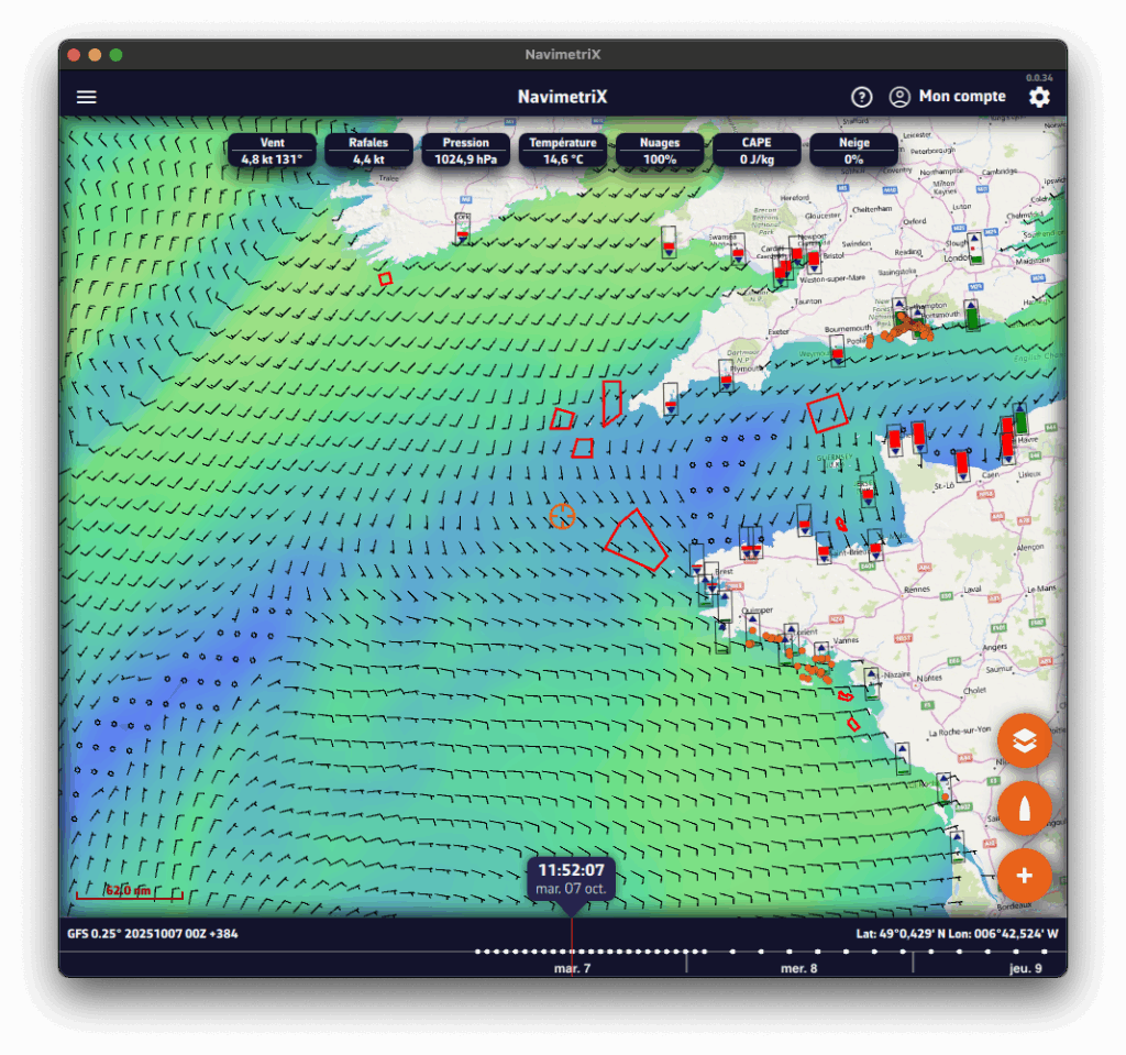
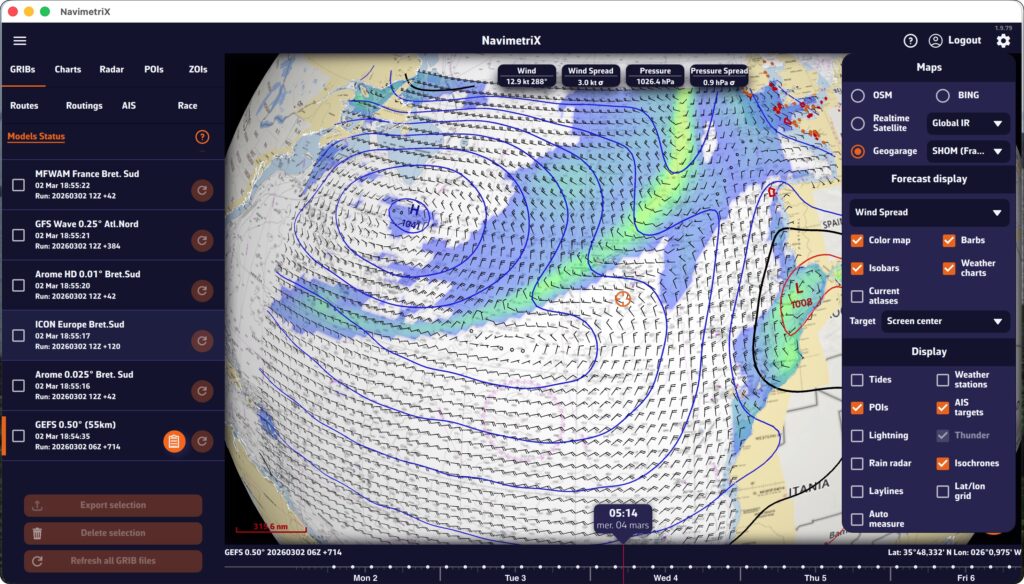
The NavimetriX interface has been designed to be clear, intuitive, and quick to use, whether on a computer, tablet, or smartphone. Here is a complete description, section by section:
- Top right
- ⚙ Settings icon: opens the settings panel
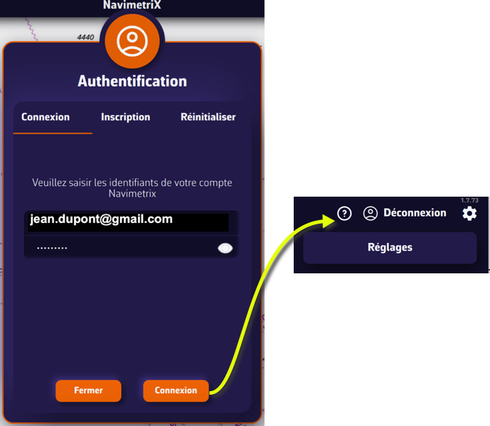
- 👤Account icon: allows you to log in to your NavimetriX account, create an account, or reset your password.
- ? Help icon : Open the application's website, in the Frequently Asked Questions or FAQs tab.
- Top left
☰ Hamburger menu: provides access to the application's main lists:
- GRIBs files
- POIs Points of Interest
- ZOIs Zones to avoid, i.e. Traffic Separation Schemes
- Routes
- Routings
- AIS targets
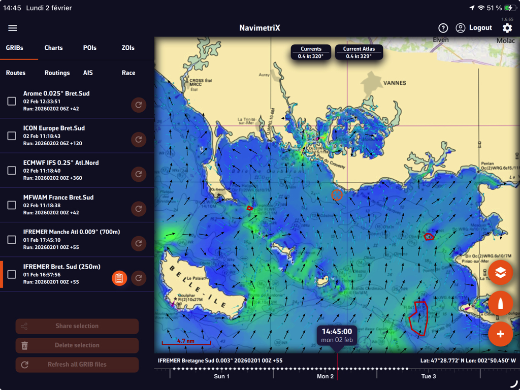
- Bottom left
- Map scale
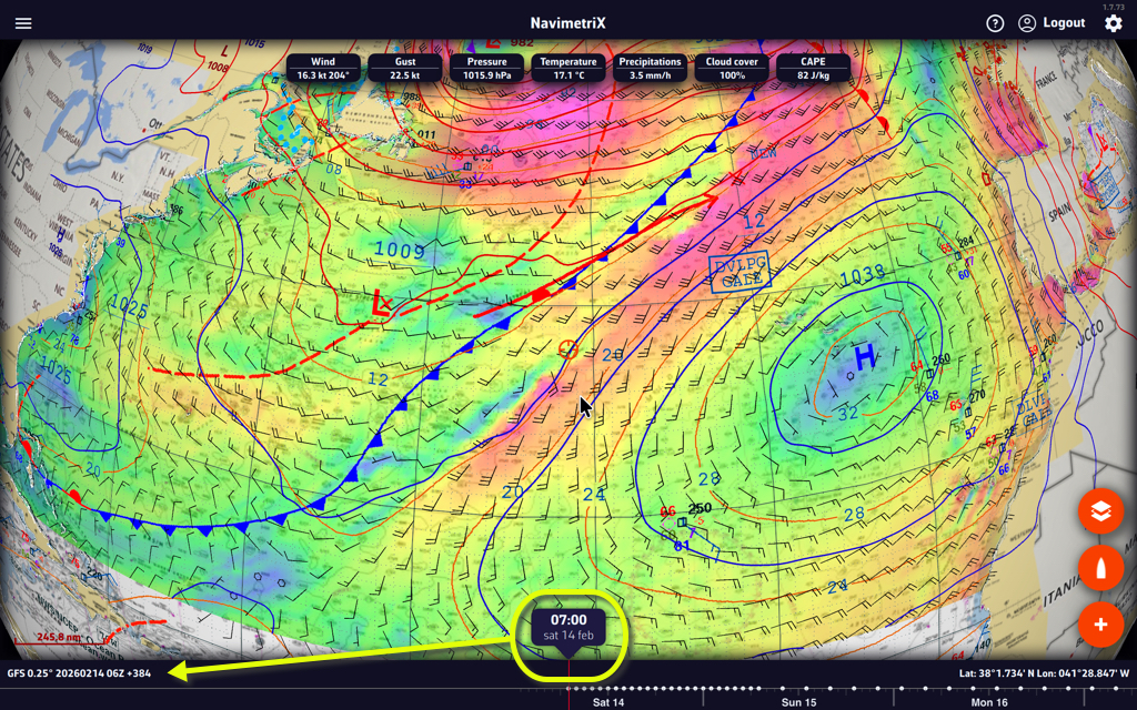
- GRIB file loaded, in example :
GFS 0.25° 20251007 00Z +384
- GFS model
- 0.25° grid, approximately 26 km
- published by NOAA on October 7, 2025
- Calculated at midnight UTC, we refer to the 0-hour run or 00Z.
- containing 384 hours from the 00Z run. If you see +36, this indicates that the first 36 hours of this GRIB file are from the 00Z run, while the following hours are from the previous run, which was the 18Z run on October 6. This gives you access to the latest data from the run without having to wait for the entire run to be calculated. For the GFS, this saves about 3 hours.
- Below: the Timeline
- Displays all hours covered by the currently loaded GRIB file.
- Each white dot on the time bar corresponds to a time step in the GRIB file.
- The time displayed just above indicates the current position of the Timeline.
- If you click/tap on this time, the Timeline will jump to “now” and the seconds will scroll by (letting you know that you are at the current time)
- You can:
- Slide the Timeline with your finger or mouse,
- Click/tap on a location to move directly to a specific time.
- The data in the GRIB file displayed is then that for the selected time.
- If a routing is displayed, the boat moves at the selected time along its trajectory.
- At the bottom right, the coordinates of the target in the center of the screen are displayed.
- Bottom right: the three orange circular buttons
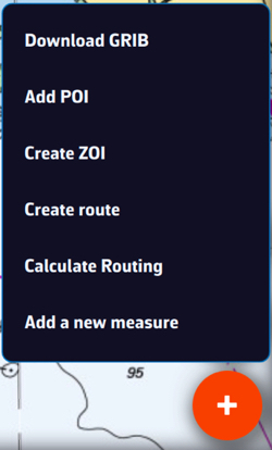
- Action Button (+)
- Download a GRIB file,
- Add a POI,
- Create a ZOI
- Create a route,
- Calculate a routing.
- Add a new measure
- Action Button (+)
- Boat Button
- Centers the map on the boat's position.
- Long press : automatically centers and zooms in for a closer view—ideal for navigation.
- Boat Button
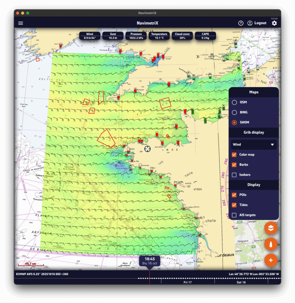
- Layers button
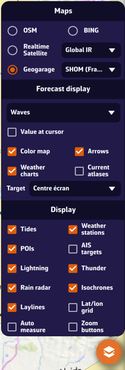
- Chart section :Allows you to choose the type of chart displayed:
- OpenStreetMap (default)
- Bing Satellite
- Realtime Satellites images
- Geogarage: Nautical charts, if available.
- Chart section :Allows you to choose the type of chart displayed:
- GRIB Display section
- Allows you to choose which weather parameters to display:
- Cursor value (PC/Mac pointer),
- Background color,
- Wind barbs,
- Isobars
- Weather maps
- Current atlases (SHOM)
- Additional data depending on the loaded model.
- Target (dropdown menu): Screen center (default), disabled, GPS location, POI.
- Allows you to choose which weather parameters to display:
- GRIB Display section
- Display Section
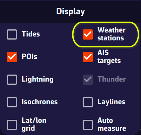
- Allows you to enable or disable the display of :
- Tides
- Weather stations
- POIs,
- AIS targets
- Lightning, Thunders
- Rain Radar
- Isochrones
- Laylines
- Lat/Lon grid
- Auto measure
- Allows you to enable or disable the display of :
- Display Section
- Layers button
- On the map
- Target in the center of the screen.
- Orange if at sea
- Blue if on the ground The target's coordinates are displayed at the bottom right.
- Target in the center of the screen.
- Data from the GRIB file at the target at the time of the time bar
- Tide icons around the world
- Red : ebb tide.
- Green : rising tide. Clicking on an icon opens the tide details with the times and heights calculated directly in the application.
- Tide icons around the world
- No-go zones
- red polygons, such as TSS (Traffic Separation Schemes) or offshore wind farm areas
- No-go zones
- Points of Interest (POIs)
- in orange
- Points of Interest (POIs)
You will find a short tutorial on the basic functions of NavimetriX by following Get Started.
PermalinkOnce the app is installed, preferably on a mobile device from the Apple Store or Google Play, you must first subscribe to the Premium subscription for the 7-day trial period.
1. Take out the Premium subscription

Tap the “Cart” icon to open the Premium subscription window. If you select the “Account” icon before subscribing, the authentication window reminds you that you must subscribe first.
If you do not wish to continue your subscription beyond 7 days, you will need to cancel it before that deadline to avoid being charged.
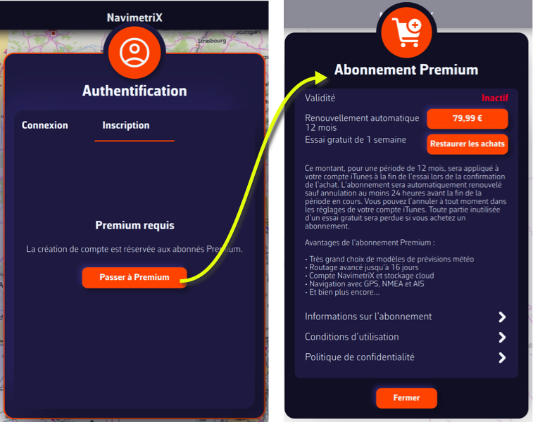
Once subscribed, the "Cart" icon disappears from the screen.
2. Create your NavimetriX account

- Tap "My Account" in the top right corner, or the icon above (for smartphones).
- Select the Sign Up tab from the Authentication menu.
- Enter an email address and a password.
- Press the orange "Request a code" button.
- Enter the code received by email, then press the "Sign Up" button.
- Then go to the Log In tab in the Authentication menu.
- Enter your NavimetriX account email address and password, and press the orange "Log In" button.
Warning: You must create your account on the device you used to purchase the Premium subscription.
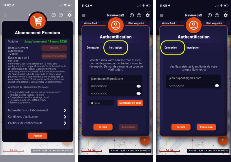
- The "My Account" button has been replaced by "Logout".
You can now enjoy all NavimetriX features for 7 days.
Warning: if you wish to continue your subscription for a year, do not cancel it before the end of the 7-day trial.
PermalinkBefore writing to us, please check the FAQs — you’ll probably find the answer to your question 😉.
There’s no need to browse through all the FAQs one by one: you can search within the FAQs, so don’t hesitate to use the search bar!
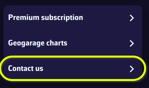
- If you are using the app, please use the “Contact us” menu option in Settings. An email will automatically be prepared with some technical data, and a "log" file in attachment (*), that will help us respond to you. Please be specific in your questions and don’t hesitate to attach screenshots.
- Otherwise, please use the contact form on this website.
(*) For Windows and macOS, if the log file isn't attached to the email, you can add it manually; it can be found here:
- Windows:
C:\Users[your username]\AppData\Local\Soft4Sail\NavimetriX\logs\navimetrix.log
- macOS:
~/Users/[your username]/Library/Containers/navimetrix/Data/Library/Application Support/Soft4Sail/NavimetriX/logs/navimetrix.log
PermalinkHow to synchronise?
In order for NavimetriX to be synchronised across two or more devices, you must:
- Have subscribed to the Premium option and created a NavimetriX account
- Have devices connected to the Internet (Wi-Fi, cellular or satellite).
- Be logged into the same NavimetriX account on all devices
Which items are synchronised and which are not?
Most settings are synchronised, with a few exceptions, namely:
Synchronised
- All application settings, except:
- The language used
- The display size percentage
- The instrument configuration (which must be fitted to screen sizes)
- Internal or NMEA GPS source (GPS & NMEA)
- With no exception
- POIs, routes, routings, routing tables, statistics, AI briefing, input data
- Screen display of charts, GRIBs, POIs, tides, AIS targets, routing isochrones
Partially synchronised
- GRIBs files


Downloaded GRIB files appear in the GRIB list on all devices. When a GRIB is downloaded or updated on a device, it is followed by a dimmed refresh icon. If a new run is available for that GRIB, this icon is activated.

On other device(s), the list of downloaded GRIBs is displayed but followed by an activated download icon. The contents of the GRIBs must then be downloaded manually.
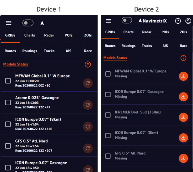
Once the GRIBs are identical on all devices, the download icon is replaced by the refresh icon.
- Geogarage charts
The Geogarage account is synchronised across all devices.
Geogarage charting is not synchronised: charts must be downloaded to each device.
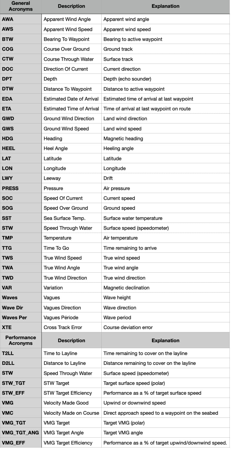
📘 This glossary brings together the main terms used in the Navimetrix application and its FAQs. It helps users better understand concepts related to navigation, routing, and marine weather. A comprehensive table is presented at the bottom of this page.
Course Over Ground (COG)
The actual direction of the boat’s movement over the seabed, expressed in degrees relative to true north. It differs from the compass heading when there is drift caused by wind or current.
Speed Over Ground (SOG)
The boat’s actual speed relative to the ground (not the water). Calculated by GPS, it includes the effect of currents.
Heading (HDG)
The direction in which the boat’s bow is pointing, measured relative to true or magnetic north.
True Wind Angle (TWA)
The angle between the boat’s axis and the true wind direction. It is calculated from the apparent wind and the boat’s speed.
True Wind Speed (TWS)
The wind speed derived from the apparent wind and the boat’s speed. It represents the actual wind strength on the sea surface.
Apparent Wind Angle (AWA)
The wind angle felt on board, influenced by the boat’s motion. Measured relative to the boat’s centerline.
Apparent Wind Speed (AWS)
The wind speed felt on the boat, resulting from the combination of the true wind and the boat’s speed.
Velocity Made Good (VMG)
The useful component of the boat’s speed, indicating the effective progress toward the destination or upwind.
Closest Point of Approach (CPA)
The point at which two vessels will be at their minimum distance from each other, based on their current courses and speeds.
Time to CPA (TCPA)
The time remaining before reaching the CPA, used for collision avoidance and AIS alarms.
Bearing
The angle between north and the direction of an observed object from the boat. Used to determine the relative position of a target or coastline.
Depth
The water depth below the keel, measured by an echo sounder. A key parameter for safe navigation.
Waypoint (POI / Waypoint)
A geographic point used to define a route or a key position. In Navimetrix, POIs represent these waypoints.
GRIB File (Gridded Binary)
A standard file format containing numerical weather forecasts (wind, waves, pressure, temperature, etc.).
Isochrone
A curve connecting all possible boat positions at a given time according to the predicted weather conditions.
Routing
The calculation of an optimal route considering wind, waves, currents, and the boat’s performance.
Polar
A performance curve showing the boat’s speed as a function of wind angle and wind strength. It forms the basis for the routing engine.
Estimated Time of Arrival (ETA)
The predicted time of arrival at the destination, calculated from the remaining distance and the average speed.
Sea State
A description of the waves and swell (height, direction, period). Used to assess routing comfort and safety.
Swell
A regular train of waves formed by distant winds. It differs from the wind sea, which is generated locally.
Significant Wave Height
The average height of the highest one-third of waves, the main indicator of overall sea conditions.
Currents
Water movements caused by tides or ocean circulation. They affect the boat’s speed and trajectory.
Tide
Variation in sea level caused by the gravitational attraction of the Moon and the Sun. It influences depth and coastal currents.
Complete acronym table
- Requirements: You must have subscribed to the Premium option and created an account on the device used to take out the subscription.
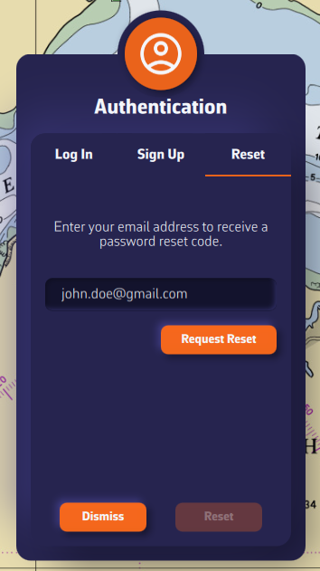
- Press “👤 My Account” at the top right.
- Go to the Reset tab in the Authentication menu.
- Enter the email address of your NavimetriX account and press Request Reset.
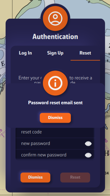
- An email is sent to your inbox — press Dismiss on the information window.
- Enter the reset code and the new password.
- Press the Reset button.
Q4 2025
- Distance measurement - ✓
- Edit zones (restricted, slow, info) - ✓
- Isobar redesign - ✓
- Display of all weather parameters - ✓
- Route plan - ✓
- Data along the routing - ✓
- Meteogram in grid format - ✓
- Alarms - ✓
- Multi-GRIB routings - ✓
- “In situ” data - ✓
- NKE interface - ✓
- Autopilot control interface - ✓
- Laylines - ✓
- Demo mode - ✓
Q1 2026
- Linux - ✓
- Multi-GRIB routing - ✓
- Route tracking - ✓
- Race tracking - ✓
- AIS over Internet - ✓
- NMEA over USB - ✓
- Import third party GRIB files - ✓
- SHOM currents atlases - ✓
- Automatic Routing Playback (Play button) - ✓
- Timeline extension - ✓
Q2 2026
- Satellite images - ✓
- Isobaric charts - ✓
- Rain Radar - ✓
- Real-time storm tracking - ✓
- "In situ" stations - ✓
- Ensemble routing - ✓
- Advanced track management - ✓
- Safe Mode
- Automatic local backup
Q3 / Q4 2026
- Synchronized anchor watch - ✓
- Assisted GRIB download (Magic wand) - ✓
- Analog instruments
- Full screen mode
- Dual-screen mode
- CMap charts
- Avurnav
- ENC charts
- Local network synchronization
- Navigator
- Wave modeling
- Polar creation and editing
- Sail configuration creation and editing
- Navigation sharing
Despite NavimetriX's constant focus on optimisation, the wide variety of devices that can be used makes it impossible to guarantee optimal performance in every case. The prerequisites stated in the FAQ (1) are sometimes not enough, as technical specifications can be limiting on certain device ranges. It is therefore advisable to take precautionary measures to minimise the malfunctions that may be encountered.
Unexpected closure on launch or during use
An immediate closure on launch is often caused by a large number of saved routings that are reloaded at every start-up. This can be enough to cause the application to close immediately after opening by instantly saturating the RAM.
Only keep routings currently in use, especially if you are running ensemble routings, which are very heavy, as they are stored on our servers for synchronisation. A routing is only valid for the lifetime of the weather models it uses. Once it has expired, there is no need to keep it. If necessary, you can export it and re-import it later as a route.
RAM saturation can also cause unexpected closures during use, when launching a resource-intensive function: end of a long routing with an isochrone step that is too short or a search area that is too wide (> 220°), or an ensemble routing.
Degraded display
Sluggishness during screen interactions (zoom +/- functions, scrolling), or the appearance of black areas (partial or total loss of chart display) are often caused by RAM saturation on poorly equipped devices. Make sure to close and quit unused applications to free up RAM.
Also, to improve smoothness, the heaviest layers to disable are AIS and data stations (InSitu); for the track, switch the ongoing track to “Short” (last 20 minutes) and hide saved tracks in the Tracks panel. Displaying GRIBs as particles is also graphics-intensive and drains the battery. Prefer arrow or barb display while navigating.
———
(1) See also: What are the minimum operating system versions?
PermalinkInstallation
💻 Desktop:
- macOS: Version 13 (macOS Ventura), released on October 24, 2022, and all later versions.
(x86_64, x86_64h, and arm64). - Windows: Version 10 (build 1809 - 10.0.17763) or later, Windows 11 - x86_64 and ARM64, released in October 2018.
📱 Mobile:
- Android: Version 9 (API 28) to 15 (API 35) - arm64-v8a, x86_64, x86, and armeabi-v7a. Android 9 was released in August 2018.
- iOS: Version 16 or later (including iOS 18) - armv8, arm64. iOS 16 was released in September 2022.
⚠️ Important:
These operating system versions are prerequisites for running NavimetriX, as they define compatibility with our development framework.
However, they do not guarantee that the application will be fully compatible with your device. Other factors such as insufficient RAM (*) or a low-performance graphics processor may also affect performance and compatibility.
———
(*) Regarding Windows 11, the system uses 6 GB on a PC fitted with 8 GB of RAM and more than 10 GB on a machine with 16 GB.
Permalink- Scroll down to the bottom of this page
- Click the “Get it from Microsoft” button
- Download the installation file
- Run the installation file

⚠️ If you receive a warning from your antivirus, it is most likely a false positive. The NavimetrixSetup x.x.xx.exe file is officially signed with an EV (Extended Validation) code signing certificate issued by SSL.com, on behalf of SOFT4SAIL (France).
You can check on VirusTotal that our .exe file is clean and recognized as safe by major antivirus programs.
The blocking message displayed by Windows corresponds to the “SmartScreen” protection mechanism, which can be temporarily triggered on recent or little-used applications, even when they are correctly signed. You can therefore safely authorize the application to run:
Either in the window that appears:
- Click on the “Learn more” option, then “Run anyway.”
Or by marking the file as safe:
- Right-click on NavimatrixSetup x.x.xx.exe.
- Select “Properties.”
- At the bottom of the “General” tab, check “Unblock.”
- Click “Apply” then “OK.”
- Restart the installation.
Resolving an issue on a Windows PC can be complex, given the wide variety of possible configurations. Here are some basic steps to check:
- Check the app version
- Make sure you have the latest version of the application.
The version number is displayed at the top right under the cogwheel icon. It will appear in red if your version is outdated. If you don’t see it, your version is very old. To update your app, follow this link and click the “Get it from Microsoft” button.
- Make sure you have the latest version of the application.
- Check your Windows version
- Your system must be Version 10 (build 1809 – 10.0.17763) or later, 64-bit (x86_64). See the prerequisites in the FAQ section of our website for more details.
- Your system must be Version 10 (build 1809 – 10.0.17763) or later, 64-bit (x86_64). See the prerequisites in the FAQ section of our website for more details.
- Try another network
- If you are connected to your home Wi-Fi, try using mobile data sharing (hotspot), or vice versa.
- If you are on a corporate network, make sure you are not behind a firewall that could block certain data (such as coastlines or weather data) from loading.
- If you use a VPN, disable it.
- Restart your PC
- Check our Facebook group
- Visit the Navimetrix Users Facebook Group to see if other users are experiencing the same issue.
If these steps do not solve the problem, your PC may not be compatible due to insufficient RAM or a graphics card that does not meet the app’s requirements.
PermalinkTo uninstall the application:
- Close NavimetriX
- Uninstall the application from the Windows menu “Add or Remove Programs.”
The application will be uninstalled, and all folders where it stores data as well as its registry keys will be removed.
Permalink- Uninstall the application by moving it to the Trash
- Open Finder
- Go to the directory /Users/[user]
- Show hidden files and folders in this directory by pressing "Command" + "Shift" + "." (period) simultaneously.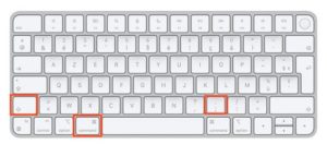
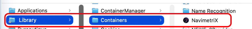
- Delete the following directory:
/Users/[user]/Library/Containers/eSail4VR
Replace [user] with your Mac username.

You can also use the CleanMyMac application.
PermalinkIf you get an error message saying “Unable to run a file from the temporary folder. Aborting installation. Error 4551: An application control policy has blocked this file” with Windows 11:
This error is caused by Smart App Control, a Windows 11 security feature that sometimes blocks the installation of new software.
To resolve the issue, you must:
- Go to Settings → Privacy and Security → Windows Security → App and browser control.
- Click Smart App Control and disable it.
- Restart the installation.
You can reactivate Smart App Control after installation.
PermalinkIf there is no Wi-Fi or USB connection to the onboard instruments, you can use a Bluetooth GPS device such as the GNS3000 from GNS Electronics. The procedure is as follows:
- Pairing the device:
- Put your GPS receiver into “pairing” mode (refer to the user manual for specific instructions; this usually involves pressing and holding a button).
- In Windows 11, go to Settings > Bluetooth & devices > Add a device.
- Select Bluetooth, choose your GPS receiver from the list, and complete the pairing process.
- Checking in Device Manager:
- Once connected, Windows usually installs the driver automatically.
- Right-click the Start button > Device Manager.
- Expand the Ports (COM & LPT) section. Your GPS should appear as a USB or Bluetooth serial port (e.g., “Standard Serial over Bluetooth link” with a COM port number, such as COM3). Note this port number.
- Using it with NavimetriX:
- Navigation applications can read NMEA data from the COM port identified in the previous step.
You should see your location data appear. If your GPS isn't detected, make sure the manufacturer-specific drivers (e.g., Garmin, Globalsat, GNS) are installed for your Windows version.
PermalinkSubscription
Once the app is installed, preferably on a mobile device from the Apple Store or Google Play, you must first subscribe to the Premium subscription for the 7-day trial period.
1. Take out the Premium subscription
Tap the “Cart” icon to open the Premium subscription window. If you select the “Account” icon before subscribing, the authentication window reminds you that you must subscribe first.
If you do not wish to continue your subscription beyond 7 days, you will need to cancel it before that deadline to avoid being charged.
Once subscribed, the "Cart" icon disappears from the screen.
2. Create your NavimetriX account
- Tap "My Account" in the top right corner, or the icon above (for smartphones).
- Select the Sign Up tab from the Authentication menu.
- Enter an email address and a password.
- Press the orange "Request a code" button.
- Enter the code received by email, then press the "Sign Up" button.
- Then go to the Log In tab in the Authentication menu.
- Enter your NavimetriX account email address and password, and press the orange "Log In" button.
Warning: You must create your account on the device you used to purchase the Premium subscription.
- The "My Account" button has been replaced by "Logout".
You can now enjoy all NavimetriX features for 7 days.
Warning: if you wish to continue your subscription for a year, do not cancel it before the end of the 7-day trial.
PermalinkWith a Premium subscription, you’ll enjoy the full potential of the application.
In addition to all the features of the free version:
- Synchronization across all your devices with a NavimetriX account: create a route on your phone, and it is instantly available on your PC
- Wide selection of weather models
- Wave and current forecasts
- Forecasts up to 15 days ahead for global models such as the U.S. GFS and the European IFS
- Routing up to 15 days
- Weather briefing generated by our AI
- Navigation mode
- Connection to onboard GPS and NMEA data
- AIS target processing
- And much more...
You’ll benefit from a 7-day free trial period, so don’t hesitate to give it a try. We’re confident you’ll be convinced.
PermalinkThe Premium subscription is annual and renews automatically.
The price depends on the region where you subscribe.
For example, it is:
- 70 GBP in the UK
- $80 in the US
- €80 per year in mainland France.
Please note that the subscription does not include nautical charts. To navigate with marine charts, you need to have a subscription on the Geogarage platform.
PermalinkAt the moment, you cannot subscribe directly from a Windows PC. To get a subscription, please use your phone (or tablet) via the App Store for iOS or macOS, or the Play Store for Android.
This subscription will then be valid on all your devices, including your PC.
When renewing a subscription or at the end of the trial period, in order to update our database with the information provided by the App Store, you must launch the application on the device that took out the subscription.
Important: On your PC or any device where you did not take your subscription, make sure to login to your NavimetriX account to see your subscription
• Cancel your subscription on the Apple Store (iOS/iPadOS):
Cancellation is done through your Apple account.
To turn off an automatically renewing subscription on an Apple device (iOS/iPadOS):
Settings > Your Account > Subscriptions > Select the subscription > Cancel Subscription
• Cancel your subscription on the Apple Store (macOS):
To cancel a subscription on a Mac, follow this link.
Note: Do not cancel before the end of the 7-day free trial if you wish to keep Premium access. However, if you do not want to subscribe, you must cancel before the end of the 7th day to avoid being charged.
• Cancel your subscription on the Google Play Store (Android):
Cancellation is done through your Play Store account.
To turn off an automatically renewing subscription on an Android device:
Follow the instructions on this page.
Note: Do not cancel before the end of the 7-day free trial if you wish to keep Premium access. However, if you do not want to subscribe, you must cancel before the end of the 7th day to avoid being charged.
PermalinkYes, this is possible thanks to the Google Play Family Library (family sharing).
NavimetriX supports Google Play family sharing. Your Premium subscription can be shared with the members of your family group, each with their own Gmail address.
Four solutions depending on your situation:
- Google Play Family Library (different Gmail addresses within a family) - Create a family group on Google Play, then add your family members. Once added, they will be able to access your NavimetriX Premium subscription on their own Android devices. See Google's help: Share Google Play content with your family.
- Same Gmail account on several devices - If you want to use NavimetriX Premium on several of your own Android devices, sign all of them in with the same Gmail account (the one that purchased the subscription).
- Two subscriptions with the same NavimetriX account - You can also purchase a subscription on each Gmail account (two subscriptions on the Play Store) and use the same NavimetriX account on all your devices. This way, your settings, routes, and points of interest stay synchronized.
- To use NavimetriX Premium on other platforms (iOS, macOS, Windows, or Linux) - Create a NavimetriX account in the app after subscribing, then sign in to that same account on your other devices. The subscription will be recognized regardless of the platform.
To create your NavimetriX account, see the FAQ "How do I log in to my NavimetriX account?".
PermalinkYes, this is possible thanks to Apple Family Sharing.
NavimetriX supports Family Sharing. Your Premium subscription can be shared with up to 5 family members, each with their own Apple ID, as long as they belong to your Apple Family group.
Three solutions depending on your situation:
- Apple Family Sharing (different Apple IDs within a family) - Set up Family Sharing in Settings > [your name] > Family Sharing, then add your family members. Once added, they will automatically have access to your NavimetriX Premium subscription on their own Apple devices. See Apple's help: Set up Family Sharing.
- Same Apple ID on several devices - If you want to use NavimetriX Premium on several of your own Apple devices (iPhone, iPad, Mac), sign all of them in with the same Apple ID (the one that purchased the subscription).
- To use NavimetriX Premium on other platforms (Android, Windows, or Linux) - Create a NavimetriX account in the app after subscribing, then sign in to that same account on your other devices. The subscription will be recognized regardless of the platform.
To create your NavimetriX account, see the FAQ "How do I log in to my NavimetriX account?".
PermalinkSettings
In the Settings panel, the first section covers the basic configuration options:
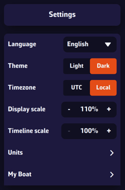
- Language: French, English, German, Spanish
- Theme: light or dark user interface
- Time zone: local (based on your device) or UTC (Universal Time)
- Display scale: allows you to decrease or increase the size of the objects on the map.
- Timeline scale: allows you to decrease or increase the default zoom level according to your screen size.
- Units: choose according to your preferred measurement system.
- My boat: all parameters related to your vessel — polar, name, type, MMSI, etc.
Some settings are essential — both for safety and for the proper functioning of the application.
- Enable GPS to “Always”
- On iPad / iPhone: Device Settings > Apps > NavimetriX
- On Android: Device Settings > Location = On > App Permissions > Location > Allow app while using. (N.B. NavimetriX forces location to remain active in “Navigation” mode.
- Disable the device unlock code
You and your crew members must be able to access the navigation app instantly, whatever the situation. At sea, a code is useless — even dangerous if you are unable to handle navigation yourself: your crew must be able to take over quickly.
- Disable automatic sleep mode
- On iPad / iPhone: Settings > Display & Brightness > Auto-Lock = “Never”.
- On Android devices: Settings > Display > Screen timeout = from 0 to 30 minutes depending on the brand and model — unfortunately, “Never” is rarely available. Set it to the maximum possible time.
Unexpected sleep mode during a critical navigation moment (e.g., nighttime landfall in the rain in an unknown area) can be dangerous if you cannot instantly relaunch the app (e.g., wet fingers or touchscreen not responding). You should manually activate or deactivate your screen depending on the situation.
- Disable spell checking
- On iPad / iPhone: Settings > General > Keyboard > Auto-Correction = disable.
- On Android devices: Settings > General Management > Samsung Keyboard Settings > Auto spell check = disable.
This prevents wasting time when entering text in the app, such as route names, POIs, etc.
Regarding onboard computers, PC or Mac, the same recommendations apply. Adjust the settings according to the operating system and version used.
Permalink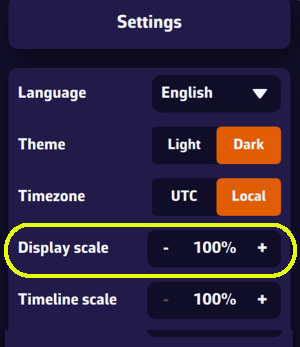
This setting allows you to enlarge or reduce the size of all elements displayed on the map (from -60% up to 200%). Very useful on board if you want to use the app without wearing your glasses.
Note that the menu font size remains unchanged.
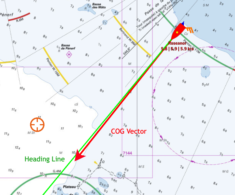
On the chart, the course vector on the ground COG is represented by a red arrow. The magnetic heading line is represented by a green line. Both are variable in length.
Open the app settings by tapping on the ⚙︎ icon, then select the My Boat section.
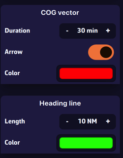
- The length of the heading vector is defined in minutes of time, from 0 up to 300mn. In example, 30 minutes on course at a 6 knots speed displays a vector of 3 nautical miles. This vector varies depending on your speed. You can disable the arrowhead.
- The heading line is set by distance on the chart, from 0 up to 300 NM. In example 20 nautical miles.
Procedure:
<li>Close <strong>NavimetriX</strong>.</li>


<li>Right-click the NavimetriX shortcut (or the <code>NavimetriX.exe</code> file in its installation folder).</li>


<li>Select <strong>Properties</strong>.</li>


<li>Open the <strong>Compatibility</strong> tab.</li>


<li>Click <strong>Change high DPI settings</strong>.</li>


<li>Check the option:<br><em>Override high DPI scaling behavior.</em></li>


<li>In the dropdown menu below, choose <strong>Application</strong>.</li>


<li>Click <strong>OK</strong>, then <strong>Apply</strong>.</li>


<li>Restart <strong>NavimetriX</strong>.</li>


<li>Text and interface elements should now appear larger.</li>
By default, the target is placed in the center of the screen, allowing you to drag the map underneath it and use the zoom to position it at a specific location.
However, you can lock the target to other elements, or even disable it.

Tap/click on the layers button.
In the “Target” drop-down menu, select which element you want to lock the target to:
- Disabled (to remove the target from the screen)
- Screen center (to place it to its original location)
- GPS position (to place it on your boat)
- A POI
You can also lock the target onto a POI by editing it.
Note: the edit option is only accessible when a GRIB is displayed.
PermalinkWeather
A GRIB file (for GRIdded Binary) is a standard file format used by meteorological services to distribute numerical weather forecasts.
It contains the raw data generated by weather models (wind, pressure, rain, waves, currents, etc.) organized on a grid covering a geographic area.
Why use this format?
- It is compact: GRIB files are compressed and therefore quick to download, even with limited internet connections.
- It is standardized: most navigation and weather applications can read GRIB files. There are two formats — grib1 and grib2. NavimetriX uses the newer grib2 format.
- It is flexible: you can choose the area, resolution, and parameters (wind, waves, currents, etc.) you wish to download.
What does a GRIB file contain?
Depending on the selected model, a GRIB file may include:
- Wind (direction, speed, gusts)
- Atmospheric pressure
- Temperature, humidity, precipitation
- Sea state (swell, waves)
- Marine, oceanic, and tidal currents
What is it used for in navigation?
A GRIB file allows you to visualize the evolution of the weather over a given area directly within your navigation software or weather app.
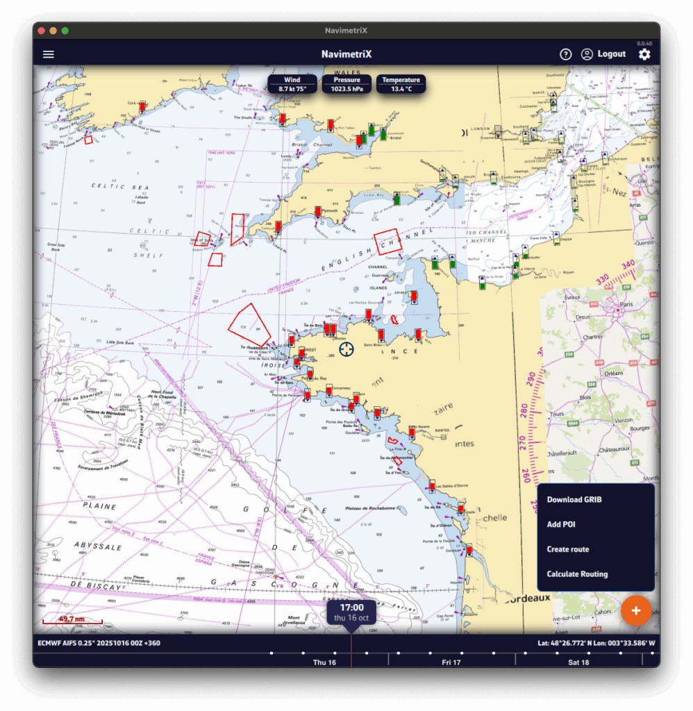
PermalinkTo illustrate the process, let’s say we’re planning a 4-day passage from La Rochelle (France) to Cowes (UK).
- Pan and zoom to your sailing area. Unless you’re doing an ocean crossing, pick a selection slightly larger than your route.
- Press the + button.
- Tap Download GRIB.
- If needed, adjust the selection using the four green corners.
- Press OK.
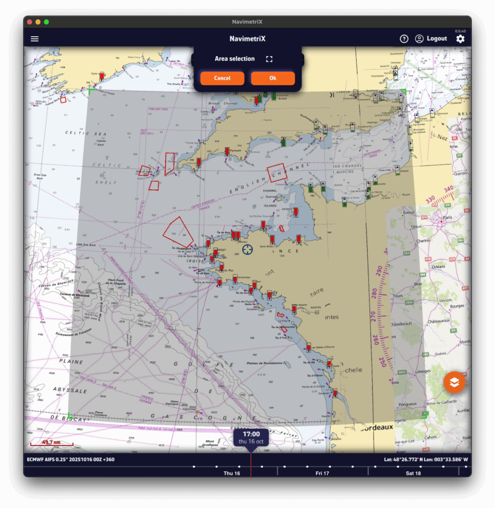
A Download GRIB window opens. The choices are filtered to your selected region.
Without the Premium option, you’re limited to the GFS model (the U.S. NOAA global atmospheric model).
- Choose the Type of data to download:
- Atmospheric
- Current
- Sea State
- Choose the Coverage:
- Global
- Regional — for trips up to ~5 days, a regional model is usually best.
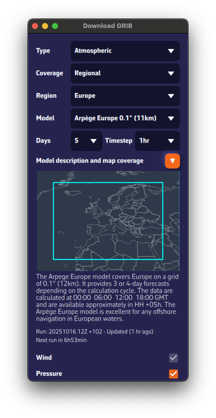
- If applicable, select the Region.
- Select the Model.
See our FAQs for guidance on models.
If unsure, choose the atmospheric global ECMWF IFS or GFS. - If needed, check the Model description & coverage map.
- Select the Days and Timestep.
If unsure, keep the defaults. - Choose the Parameters (Wind, Pressure, etc.).
If unsure, keep the defaults.
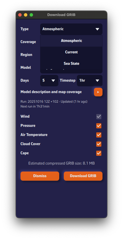
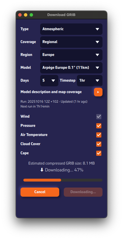
The estimated compressed GRIB size appears at the bottom. Keep it reasonable—if you see ~200 MB, you probably chose a model that’s too fine or too many parameters.
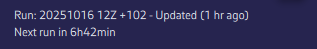
Below the model description, we show the latest model calculation time (the Run).Run: 20251016 12Z +102 means: calculated on Oct 16, 2025; initialized at 12:00 UTC (12Z); contains 102 forecast hours from that run.
We also display the estimated time until the next run is available.
- Press Download GRIB.
- The GRIB file downloads from our fast, redundant servers.
- Once downloaded, it is:
- displayed on the map. If you don’t see it, open Layers and enable Color map and Barbs.
- added to the GRIB list in the left panel. Tap the ☰ at top-left to open the lists panel.
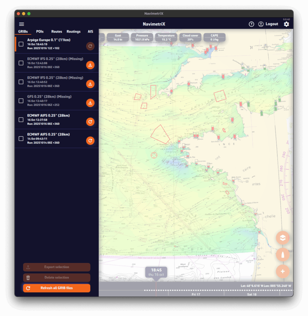
You may have noticed a small icon on the right of each item in the GRIB files list. This icon shows the update status of your GRIB file and can display three different states:
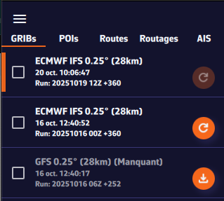
1. Dark orange “Refresh” icon — file up to date
The icon appears in dark orange right after a GRIB file has been downloaded. This means your file is up to date — you already have the latest available version of the weather model.
This is what you will see immediately after downloading a GRIB file.
2. Light orange “Refresh” icon — new run available
The icon turns light orange. This means a new model run (a new forecast) is available. To update your GRIB file, simply click or tap on this icon: the file will automatically be replaced with the latest version.
3. Light orange icon with a download symbol — file missing on this device
Finally, the icon may appear in light orange with a small download symbol. This means you have already downloaded this GRIB file on another device, but it is not yet available locally on the one you are using. To retrieve it, simply click or tap on the icon: the file will be downloaded automatically.
See also: Where can I see weather models status
PermalinkGlobal models (such as GFS or ECMWF) cover the entire planet. They are essential for long crossings and long-term forecasts (up to 10–15 days), but their resolution remains limited (20 to 50 km). They are used to get an overall view of the weather and for long-distance passages.
Regional models focus on a specific area (France, Europe, the Mediterranean…). Their coverage is smaller, but their resolution is much finer (2 to 10 km), allowing for better anticipation of local effects such as thermal breezes, thunderstorms, terrain, and coastal winds. In return, they generally only extend 2 to 3 days into the future. They are used for day trips or short cruises.
If you’re not familiar with weather models, you’re probably wondering which ones to choose.
Here are a few simple rules:
Select the model according to your navigation area and type of sailing, following the table below.
For weather data, if in doubt, choose the ECMWF IFS model.
The ECMWF IFS model covers the entire globe for up to 14 days. However, note that forecast reliability decreases with time:
| Forecast range | Reliability level |
|---|---|
| Up to 2 days | Excellent |
| 2–4 days | Very good |
| 4–5 days | Good |
| 5–8 days | Reasonable trend |
| 8–10 days | Rough trend |
| Beyond | At best a trend — often unreliable. Prefer the AIFS model, computed using Artificial Intelligence. |
Here’s a table to help you choose. We’ll soon add an automatic selection feature based on your sailing program.
| Type of data | Type of navigation | France – Atlantic & Channel | France – Mediterranean | Europe (outside France) | United States | Rest of the World |
|---|---|---|---|---|---|---|
| Weather | Day sailing in a bay | Arome | Arome | UKV, ICON Europe Arpege Europe | NAM HRR Conus | ECMWF IFS |
| Weather | Coastal | Arpege Europe | Arpege Europe ICON Europe | UKV, ICON Europe Arpege Europe | NAM HRR Conus | ECMWF IFS |
| Weather | Offshore | ECMWF IFS and AIFS GFS | ECMWF IFS and AIFS ICON Europe | ECMWF IFS and AIFS GFS | ECMWF IFS and AIFS GFS | ECMWF IFS and AIFS GFS |
| Waves | Coastal | MFWAM France | MFWAM France | MFWAM Global | GFS Wave | GFS Wave |
| Waves | Offshore | MFWAM + GFS Wave | MFWAM Global | MFWAM Global GFS Wave | MFWAM + GFS Wave | MFWAM + GFS Wave |
| Currents | Day sailing in a bay | Ifremer | Copernicus Med | Copernicus | MSC NCOM | Copernicus SMOC |
| Tidal currents | Coastal | Copernicus IBI | Copernicus Med | Copernicus IBI or ENWS | MSC NCOM | Copernicus SMOC |
| Ocean currents | All | Copernicus IBI | Copernicus Med | Copernicus IBI or ENWS | Copernicus Global | Copernicus Global |
- Arpege Europe 0.1° (11 km)
Regional model from Météo-France covering Europe and extending down to the Canary Islands.
Resolution: 11 km
Forecasts up to 4 days
👉 Ideal for planning navigation in the Channel, Atlantic, or Mediterranean over a few days, as it accurately captures large-scale European weather systems.
- Arome 0.025° (3 km)
Very high-resolution model from Météo-France.
Resolution: 3 km
Forecasts up to 48 h
👉 Perfect for coastal navigation in France: it captures local effects such as sea breezes, summer storms, and terrain-induced winds.
- Arome HD 0.01° (1 km)
Even higher-resolution version of Météo-France’s Arome model.
Resolution: 1 km
Forecasts over 24 h
👉 Very useful for racing or coastal sailing: it helps anticipate micro wind shifts near capes, bays, or coastal terrain. Be aware, it can sometimes be a bit “reactive.”
- ICON Europe 0.07° (8 km)
Regional model from the DWD (German Meteorological Service).
Resolution: 8 km
Forecasts up to 5 days
👉 Suitable for navigation in the English Channel, North Sea, Western Mediterranean, and nearby Atlantic. A good complement to French models and often cited as the best in the Mediterranean.
- ICON D2 0.02° (2 km)
Very high-resolution version of the ICON model, centered on Germany and neighboring countries.
Resolution: 2 km
Forecasts up to 48 h
👉 Useful for the North Sea and Baltic Sea, where local effects (coastal winds, thunderstorms) are significant.
- UKV 0.05° (6 km)
Regional model from the UK Met Office, covering the United Kingdom and nearby areas.
Resolution: 6 km
Forecasts up to 48 h
👉 Ideal for sailing around the British Isles, in the Channel, and in the Celtic Sea, where local precision is essential.
Wave settings
Open the Settings panel by tapping the gear icon at the top right of the toolbar, then select Forecast display.
- Wave display
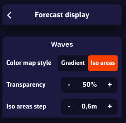
In the "Waves" section, select the Iso zones colour style, which represents wave height data as isopleth bands of equal height, using rainbow colours from blue (calm sea) to magenta-red (rough to very rough sea), passing through various shades of green, yellow, orange and red. Particularly well suited for wave data.
Transparency lets you adjust the colour mask depending on the background (satellite planisphere or nautical chart).
Iso zone step lets you adjust the spacing of the isopleth bands relative to the data type (e.g. in 0.60 m increments).
Displaying waves
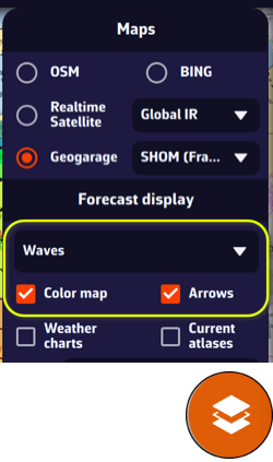
On the chart, the Layer button at the bottom right of the screen lets you choose what to display.
In the Forecast display section, the drop-down menu lets you select a data layer to display. If you have loaded a wave GRIB file on screen (for example an MFWAM model), the Waves data will be selected by default. You can toggle the display of the colour fill and barbs according to your previous settings (see above), and optionally isobars (lines of equal atmospheric pressure).
This section automatically adapts to the type of GRIB file currently displayed: weather, waves, or currents.
Permalink- ECMWF IFS 0,1° (9 km) 0.25° (28 km), 0.4° (44 km), 1° (111 km)
Global model from the European Centre (ECMWF). Often considered the most reliable for medium-range forecasts.
Resolution: from 29 km up to 111 km
Forecasts up to 10 days
👉 A key reference for offshore navigation. Prefer the high-resolution version (0,1°) for a small area, (0.25°) with a good connection for a larger area, or a lighter version (0.4° or 1°) when bandwidth is limited and the area very large.
- ECMWF AIFS 0.25° (28 km), 1° (111 km)
Brand-new model from the European Centre (ECMWF) using artificial intelligence. - Resolution: 28 km or 111 km
- Forecasts up to 10 days
- 👉 Interesting for testing AI model performance and having an alternative to traditional models. Improving day by day — already likely better than ECMWF IFS and GFS for forecasts beyond 7 days.
- GDPS (GEM) 0.15° (17 km)
Global model produced by Environment Canada. One of the finest-resolution global models available.
Resolution: 17 km
Forecasts up to 10 days
👉 Relevant for North Atlantic crossings and high-latitude sailing near the Arctic.
- ICON Global 0.25° (28 km)
Global model from DWD (German Meteorological Service).
Resolution: 28 km
Forecasts up to 7 days
👉 A solid alternative to GFS and ECMWF IFS, particularly for sailing in Europe and the Mediterranean.
- Arpege Global 0.25° (28 km)
Global model from Météo-France.
Resolution: 28 km
Forecasts up to 10 days
👉 Useful for offshore sailing near France, in the Atlantic or Mediterranean, as it is well tuned for these areas.
These models provide a simplified description of the sea state.
In short, they include the significant height of the total sea, its period, its direction, as well as the same information for the wind sea.
They are mainly used in routing when conditions are challenging.
Global Models
- GFS 0.25° (28 km), 0.5° (56 km), 1° (111 km), 2° (222 km)
Global model from NOAA (United States). Available in several resolutions: the finer the grid, the larger but more accurate the file.
Resolution: from 28 km to 111 km
Forecasts up to 16 days
Time step: 3 hours
A key reference for offshore navigation. Prefer the fine version (0.25°) with a good connection, or a lighter version (1° or 2°) when bandwidth is limited. - MFWAM Global 0.1° (12 km), 0.5° (56 km), 1° (111 km)
Global model from Météo-France. Available in several resolutions.
Resolution: from 12 km to 56 km
Forecasts up to 4 days
Time step: 3 hours
The most accurate of the global models, but limited to 4-day forecasts.
Regional Models
- MFWAM France 0.025° (3 km)
Regional model from Météo-France.
Covers the French metropolitan coasts.
Grid: 0.025° x 0.025° (3 km x 3 km)
Total forecast range: 4 days
Time step: 3 h
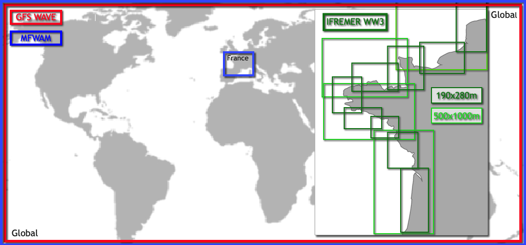
Excellent for coastal navigation. - IFREMER WW3 0.006° (500 m)
Regional models from IFREMER with several variants: North and South Channel, and North and South Gascogne.
Covers the Channel and Atlantic coasts of mainland France.
Grid: 0.004° x 0.006° (500 m x 1 km)
Total forecast range: 2 days
Time step: 1 h - IFREMER WW3 0.003° (250 m)
Local models from IFREMER with several variants:
Pas-de-Calais, Normandy-Cotentin, Armor, Finistère, South Brittany, Loire, Charentes, and Aquitaine.
Covers the Channel and Atlantic coasts of mainland France.
Grid: 0.002° x 0.003° (250 x 500 m)
Total forecast range: 2 days
Time step: 1 h
The most accurate wave model — a must when sailing through tricky coastal areas.
Weather Models
European Atmospheric Models
American Atmospheric Models
Wave Models
Current Models
See also: It’s great to have all these models — but which one should I choose?
PermalinkWind Settings
Open the Settings panel by tapping the cogwheel at the top right of the upper ribbon, then select GRIB Display.
- Wind Display
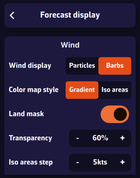
In the “Wind” section, select Particles or Barbs. Animated particles show the wind flow but consume more system resources and therefore battery — best avoided while sailing. Vectors and barbs are the classic meteorological representation of wind direction and strength. They are positioned on each grid point of the GRIB file and are more resource-efficient.
The Gradient style represents wind strength using a rainbow color scale — from blue (light or calm winds) to magenta (strong winds), through shades of green, yellow, orange, and red. Especially suitable for wind data.
The Isoplane style displays the data with the same colors but as equal-value zones. This style is better suited for data such as wave height, for example in 50-cm increments.
The Land Mask displays data over land as well. This is particularly useful when sailing among islands, to keep a continuous sea/land display.
Transparency allows you to adjust the color overlay depending on the background (satellite map or nautical chart).
The Iso-zone step adjusts the spacing between isoplane zones depending on the type of data (waves, precipitation, temperature, etc.).
Wind Display
On the map, the Layer button at the bottom right of the screen lets you choose what to display.
In the GRIB Display section, the drop-down menu allows you to select which data to display. If a weather GRIB (for example an IFS model) is displayed, Wind will be selected by default. You can enable or disable the color background, particles or barbs (according to your previous setting above), and isobars (lines of equal atmospheric pressure).
If you have displayed a wave GRIB file, you can enable or disable the color background and the wave direction arrows.
This section automatically adapts to the type of GRIB file displayed on the screen: weather, waves, or currents.
PermalinkBy default, when you display an atmospheric GRIB file on the map, wind is shown (barbs or particles, with the colour gradient). But your GRIB file contains many other parameters: precipitation, cloud cover, temperature, pressure, gusts, CAPE, etc.
To change the parameter displayed as a colour overlay on the map:
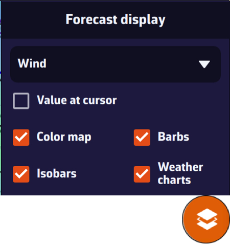
- Tap the Layers button (layers icon at the bottom right of the screen).
- In the panel that opens, find the Forecast display section.
- Tap the dropdown menu (showing "Wind" by default) to see the full list of available parameters:
- Wind
- Gust
- Delta Gust
- Pressure
- Temperature
- Precipitations
- Cloud cover
- CAPE
- Select the desired parameter (e.g. "Precipitations" or "Cloud cover"): the map updates immediately with the corresponding colour gradient.
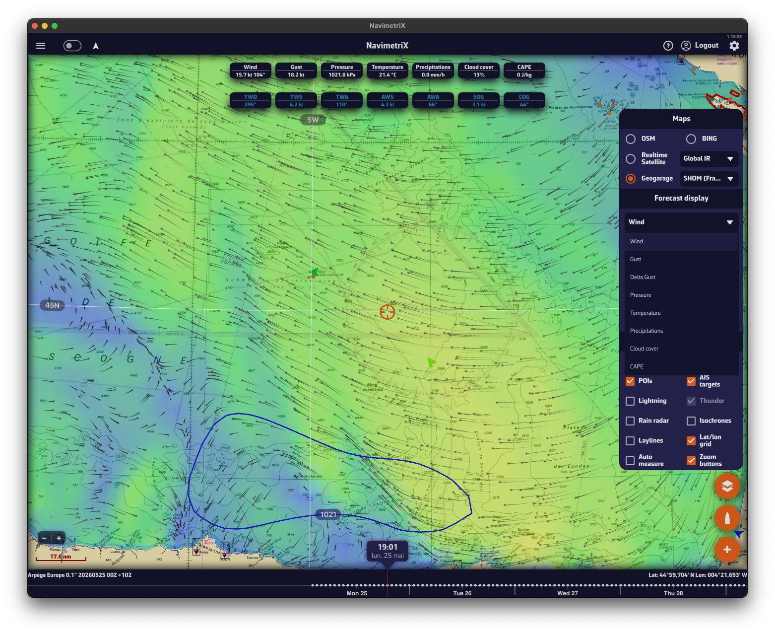
Tip: once the parameter is selected, use the timeline bar at the bottom of the screen to scroll through hours and see how precipitation, cloud cover or any other parameter evolves over the entire area covered by your GRIB file.
Note: the same principle applies to other types of GRIB files (waves, currents): the dropdown automatically adapts and offers the corresponding parameters (wave height, direction, period, etc.).
The parameters available in the dropdown depend on the data contained in your GRIB file. If you do not see "Precipitations" or "Cloud cover" in the list, make sure you ticked those parameters when downloading the GRIB file.
PermalinkBy default, a tide gauge is displayed on the cartography for each referenced station.
The gauge display can be disabled by opening the layers menu and unchecking the Tide box
The gauges currently display dynamically:
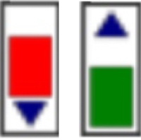
- Flow in green
- Ebb in red
Tapping on each gauge opens a tide graph showing the tide curve and the current water level, represented by the vertical timeline.
The graph is topped by a table showing the times, water heights and tidal coefficients for the day.
Tapping/clicking on the date above the table opens the calendar, allowing you to select another day/month.
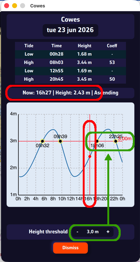
The height threshold can be used by dragging it vertically to determine:
- What the water level will be at a given time.
- What time a given threshold will be reached.
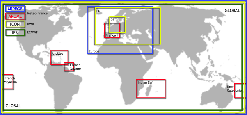
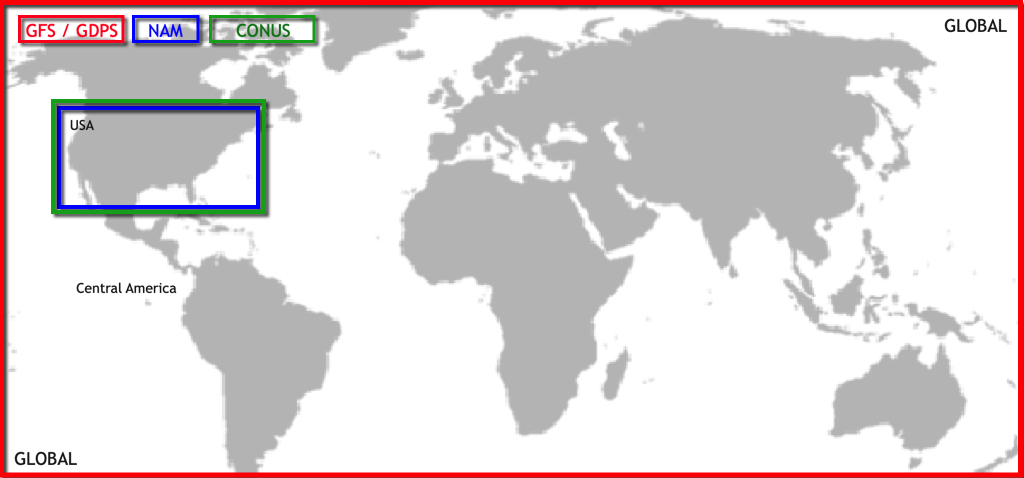
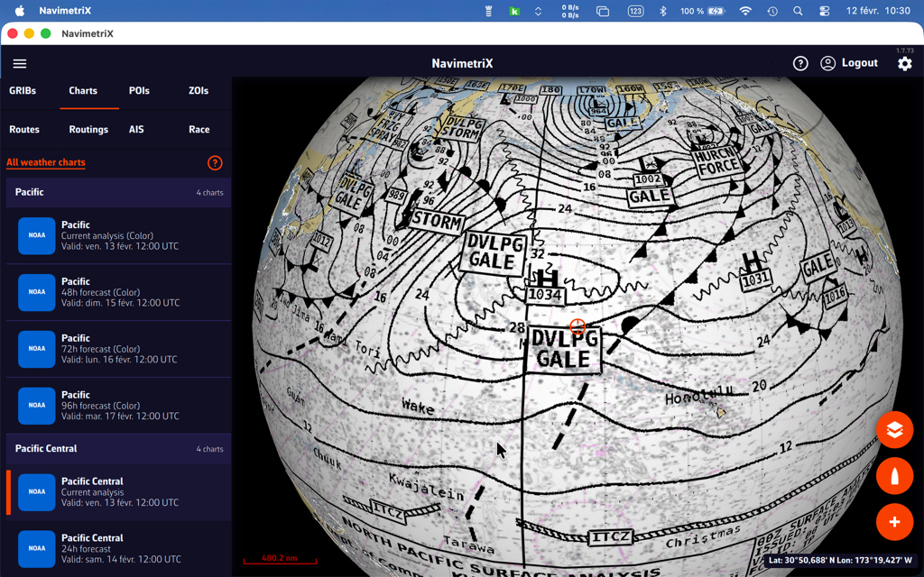
NavimetriX offers several high-resolution regional models for popular sailing destinations worldwide, in addition to global models like GFS, ECMWF, and ICON Global.
North America
NAM (11 km resolution) — NOAA's North American Mesoscale model covers the continental United States. Forecasts up to 84 hours with hourly time steps. Ideal for coastal navigation along the US East Coast, West Coast, and Gulf of Mexico.
HRRR CONUS (3 km resolution) — The High-Resolution Rapid Refresh model provides the finest resolution for the continental US. Forecasts up to 18 hours, updated hourly. Perfect for racing and detecting rapidly evolving conditions like sea breezes and thunderstorms.
Caribbean & South America
Arome Antilles (3 km resolution) — Météo-France model covering the Lesser Antilles from Puerto Rico to Trinidad. Forecasts up to 48 hours. Excellent for inter-island passages and detecting trade wind variations.
Arome Guyane (3 km resolution) — Covers waters off French Guiana and the nearby South American coast. Forecasts up to 33 hours. Useful for sailors transiting between the Caribbean and Brazil.
Pacific Islands
Arome Polynésie (3 km resolution) — Covers French Polynesia including Tahiti and the Society Islands. Forecasts up to 48 hours. Ideal for detecting local effects around high volcanic islands and reef passes.
Arome Calédonie (3 km resolution) — Covers New Caledonia and the Coral Sea. Forecasts up to 48 hours. Essential for navigating the lagoon system and anticipating thermal effects around Grande Terre.
Indian Ocean
Arome Réunion-Mayotte (3 km resolution) — Covers the western Indian Ocean from the Mozambique Channel to the Mascarene Islands, including Madagascar, Réunion, Mauritius, and Mayotte. Forecasts up to 48 hours. Critical for this cyclone-prone region.
Read also: Why are there global models and regional models
PermalinkNavimetriX provides access to over 70 weather, wave, and current models from leading meteorological agencies worldwide.
🌍 Atmospheric Models — Global
GFS — NOAA — 28 to 222 km — 16 days
ECMWF IFS — ECMWF — 9 to 111 km — 15 days
ECMWF AIFS — ECMWF — 28 to 111 km — 15 days
ICON Global — DWD — 14 to 111 km — 5 days
Arpège Monde — Météo-France — 28 km — 4 days
GDPS (GEM) — CMC Canada — 17 km — 10 days
🇪🇺 Atmospheric Models — Europe
Arpège Europe — Météo-France — 11 km — 4 days
Arome — Météo-France — 3 km — 42 hrs
Arome HD — Météo-France — 1 km — 36 hrs
ICON Europe — DWD — 8 km — 5 days
ICON D2 — DWD — 2 km — 48 hrs
UKV — Met Office — 6 km — 5 days
🌎 Atmospheric Models — Americas
NAM — NOAA — 11 km — 84 hrs
HRRR CONUS — NOAA — 3 km — 18 hrs
Arome Antilles — Météo-France — 3 km — 48 hrs
Arome Guyane — Météo-France — 3 km — 33 hrs
🌏 Atmospheric Models — Pacific & Indian Ocean
Arome Polynésie — Météo-France — 3 km — 48 hrs
Arome Calédonie — Météo-France — 3 km — 48 hrs
Arome Réunion-Mayotte — Météo-France — 3 km — 48 hrs
🌊 Wave Models (Sea State)
GFS Wave — NOAA — Global — 28 to 111 km — 16 days
MFWAM Global — Météo-France — Global — 11 to 56 km — 4 days
MFWAM France — Météo-France — France — 3 km — 4 days
IFREMER WW3 — Ifremer — France coasts (14 zones) — 190m to 500m — 4 days
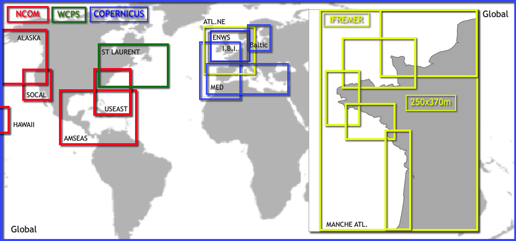
🔵 Oceanic Current Models — Global
Copernicus Global — Copernicus — 9 km — 5 days — oceanic currents only (Gulf Stream, etc.)
🔵 Oceanic and tidal Current Models — Global
Copernicus Global SMOC — Copernicus — 9 to 56 km — 5 days
🔵 Oceanic and tidal Current Models — Europe
Copernicus IBI — Iberian-Biscay-Ireland — 3 km — 5 days
Copernicus ENWS — NW Shelf / North Sea — 2 km — 5 days
Copernicus BALTIC — Baltic Sea — 4 km — 5 days
Copernicus MED — Mediterranean — 5 km — 5 days
SHOM Manche-Gascogne — Channel & Biscay — 2 km — 5 days
SHOM Méditerranée Nord — NW Mediterranean — 2 km — 5 days
IFREMER — France coasts (10 zones) — 250m to 3 km — 4 days
🔵 Oceanic and tidal Current Models — Americas
MSC Saint Laurent — St. Lawrence / Atlantic Canada — 1 km — 84 hrs
NCOM Alaska - N. Calif — Alaska to N. California — 4 km — 90 hrs
NCOM Caribbean — Gulf of Mexico & Caribbean — 3 km — 90 hrs
NCOM Hawaii — Hawaii — 4 km — 90 hrs
NCOM South California — Southern California — 4 km — 90 hrs
NCOM US East Coast — US East Coast — 4 km — 90 hrs
Read also: Why are there global models and regional models
PermalinkIn order to rename a GRIB file, you have to do a long click/tap on its name. This will bring up the keyboard, allowing you to change the name:
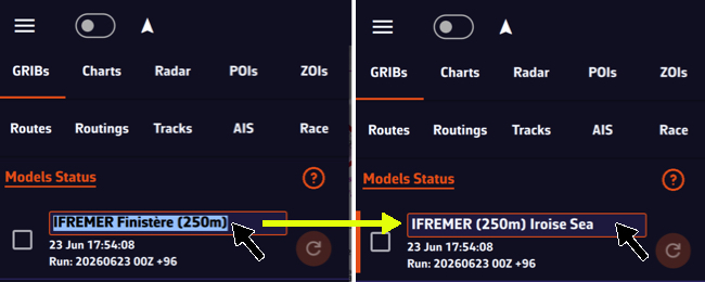
The name will be preserved during updates and synchronization.
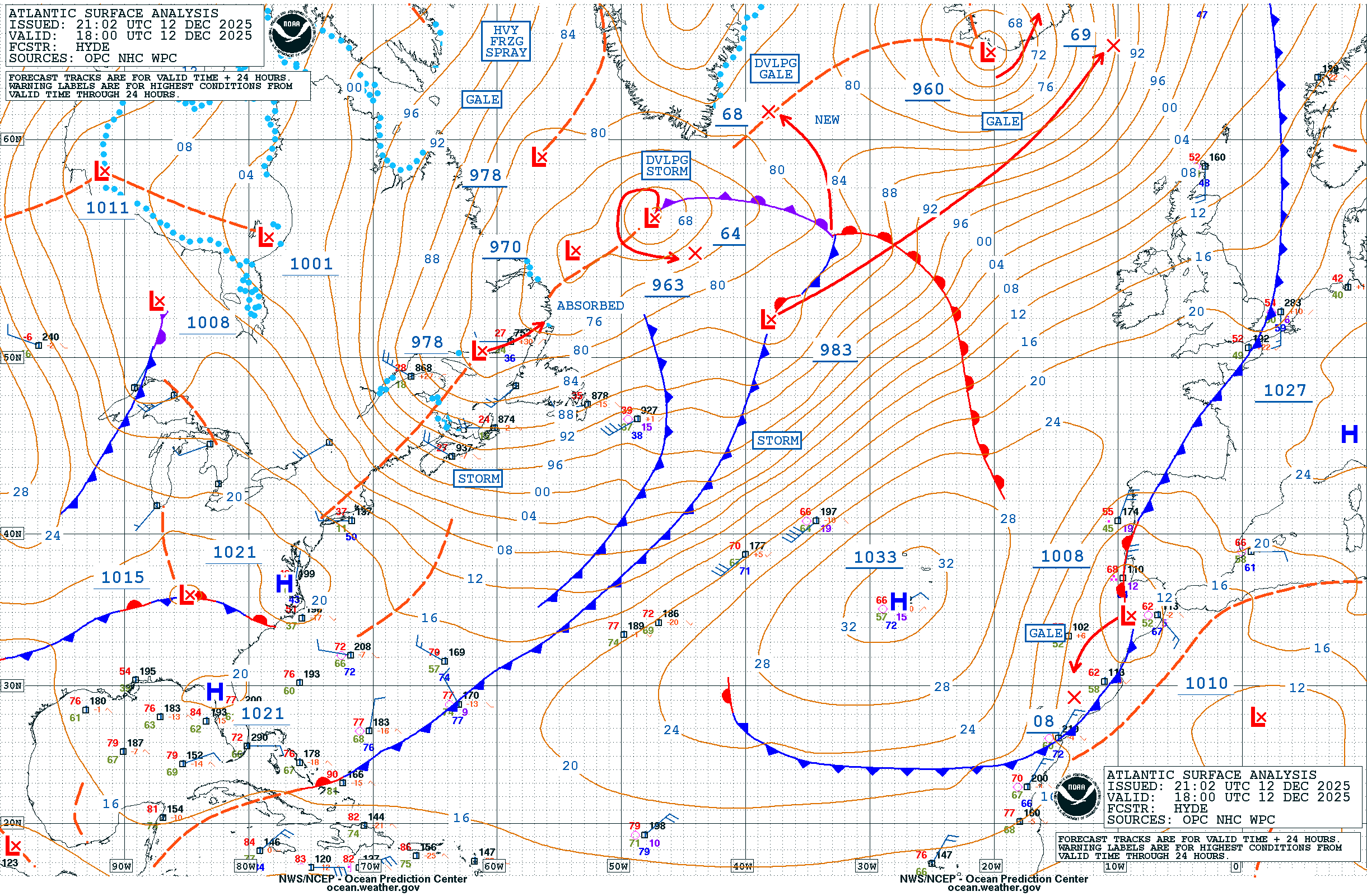
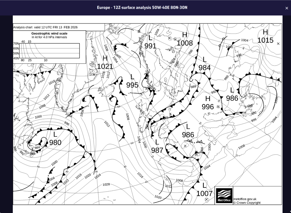
PermalinkHow to Read Marine Weather Charts (Surface Analysis Charts)
Surface analysis charts are essential tools for any sailor. They provide a synoptic view of current weather conditions and help anticipate weather changes. This guide explains how to interpret the symbols and information on these charts.
What is a Surface Analysis Chart?
A Surface Analysis Chart is a representation of weather conditions at the Earth's surface at a given time. These charts are produced by national weather services such as NOAA (USA), the Met Office (UK), or Météo-France.
They use a combination of lines, symbols, and color codes to represent:
- Pressure systems (highs and lows)
- Weather fronts
- Isobars (lines of equal pressure)
- Weather station observations
- Precipitation areas
Pressure Systems: Highs (H) and Lows (L)
Pressure systems are the main drivers of weather. They are indicated by the letters H (High pressure) and L (Low pressure).
High Pressure (H) - Anticyclone
H
Symbol: H (blue) with central pressure in millibars (e.g., 1035)
Characteristics: Air descends and spreads out, creating divergent winds. Clockwise rotation (Northern Hemisphere).
Associated weather: Generally stable conditions, clear skies, light to moderate winds, good visibility.
Low Pressure (L) - Depression
L
Symbol: L (red) with central pressure in millibars (e.g., 995)
Characteristics: Air converges toward the center and rises, creating clouds. Counter-clockwise rotation (Northern Hemisphere).
Associated weather: Unsettled weather, clouds, precipitation, strong winds. The lower the pressure, the more intense the storm.
💡 Navigation tip: A low with pressure below 980 mb is considered deep. NOAA charts sometimes indicate "GALE" (34-47 knots), "STORM" (48-63 knots), or "HURRICANE FORCE" (≥64 knots) near intense lows.
Isobars: Lines of Equal Pressure
Isobars are the thin lines connecting points of equal atmospheric pressure. They are typically spaced 4 millibars apart (1008, 1012, 1016, 1020 mb, etc.).
Key rule: Isobar spacing indicates wind strength:
| Closely spaced isobars | → | Strong gradient = Strong winds |
| Widely spaced isobars | → | Weak gradient = Light winds |
💡 Buys-Ballot's Law: In the Northern Hemisphere, if you stand with your back to the wind, low pressure is always on your left. Wind blows parallel to isobars (with a slight angle toward low pressure due to friction).
Weather Fronts
Fronts are boundaries between different air masses. Their passage typically brings significant changes in temperature, wind direction, and weather conditions.
Cold Front

Symbol: Blue line with triangles pointing in the direction of movement
Description: Cold air mass pushing into warm air. Cold fronts move faster (25-30 knots) because the denser cold air undercuts the warm air.
Weather at passage: Thunderstorms or intense but brief showers, rapid wind shift (SW → NW), sharp temperature drop, quick clearing after passage.
Warm Front

Symbol: Red line with half-circles pointing in the direction of movement
Description: Warm air mass sliding over cold air. Slower (10-15 knots) because warm air must ride up over cold air.
Weather at passage: Prolonged steady precipitation, stratiform clouds (cirrus → altostratus → nimbostratus), reduced visibility, possible fog, gradual temperature rise.
Stationary Front
Symbol: Alternating blue triangles and red half-circles on opposite sides of the line
Description: Two air masses that aren't moving relative to each other. Can persist for several days.
Associated weather: Prolonged overcast conditions, persistent precipitation over the area, stagnant conditions.
Occluded Front

Symbol: Purple line with alternating triangles and half-circles on the same side
Description: The faster cold front catches up to the warm front. Warm air is lifted aloft.
Associated weather: Mixed conditions, varied precipitation. Significance: The low is reaching maturity and beginning to weaken.
Other Boundaries
Trough
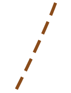
Symbol: Brown/orange dashed line in a U or V shape, often marked "TROF"
Description: Elongated area of relatively low pressure, without being a true front.
Associated weather: Atmospheric instability, wind convergence, risk of thunderstorms or unsettled weather.
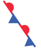
Squall Line

Symbol: Line with two red dots, often marked "SQLN"
Description: Organized line of thunderstorms, often located ahead of a cold front.
⚠️ DANGER: Violent winds, possible hail, destructive gusts. Potentially dangerous conditions for navigation!
Dry Line

Symbol: Orange/brown line with half-circles pointing toward moist air
Description: Boundary between dry continental air and moist maritime air (common in the US between Gulf of Mexico air and Southwest desert air).
Associated weather: Violent thunderstorm development along the line, especially in spring/summer.
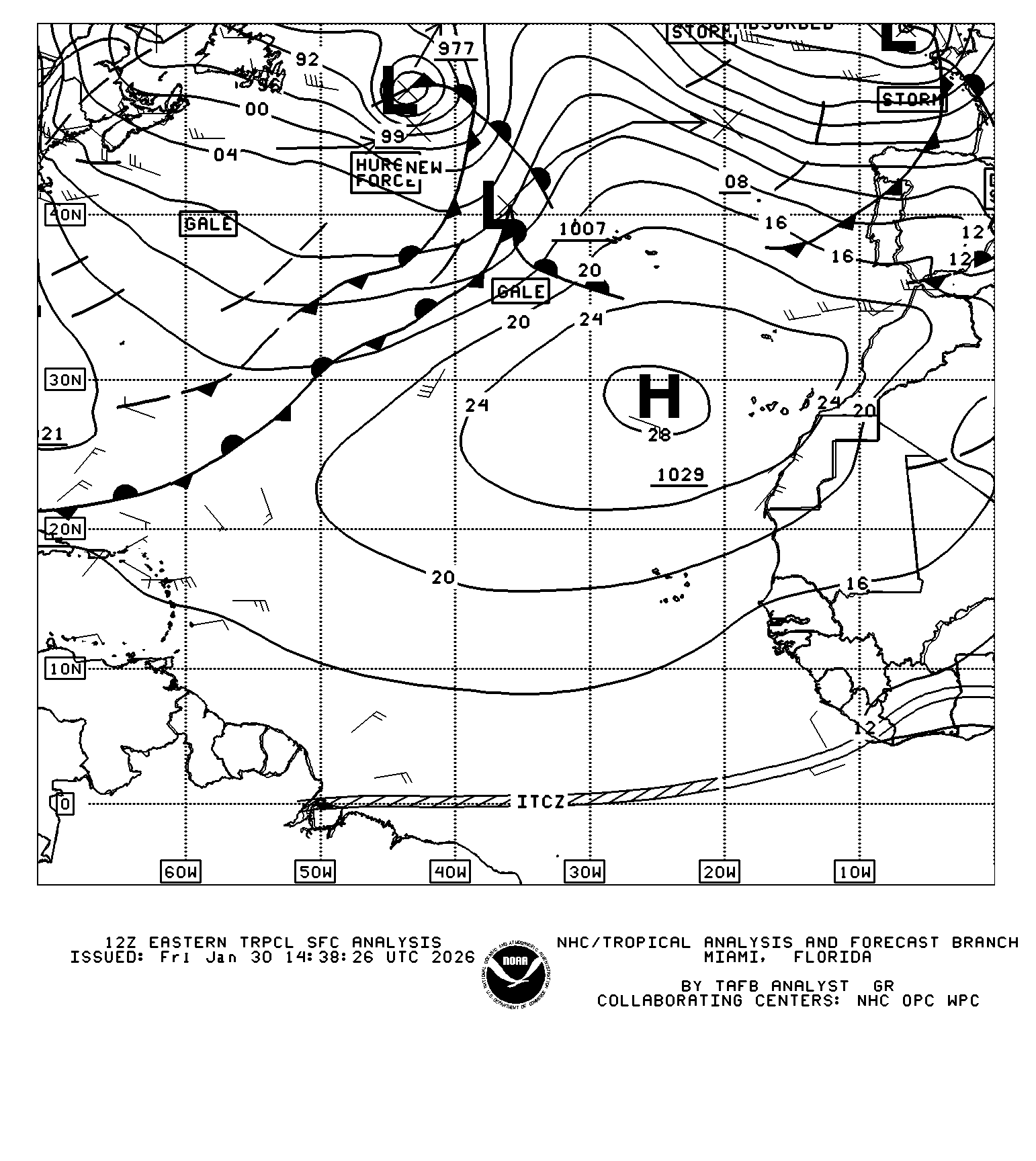
Tropical wave
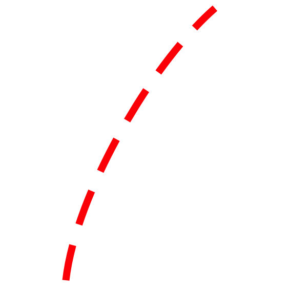
Symbol: Wide dotted red line.
Description: Rainy and stormy front moving from east to west in the intertropical zone. Frequent during the hurricane season between Africa and the Caribbean.
Associated weather: Squalls, sometimes intense, which can develop into tropical storms and then hurricanes as they progress.
📥 Complete reference: Official WPC/NOAA Front Legend
Weather Station Observations (Station Plots)
Detailed charts display weather station observations as station plots. These compact symbols summarize a lot of information at a glance.
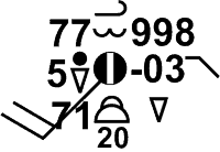
Station Plot Elements
| Position | Information |
|---|---|
| Center | Cloud cover (● overcast, ◐ partly cloudy, ○ clear) |
| Upper left | Temperature (°F or °C) |
| Lower left | Dew point |
| Right | Pressure (last 3 digits: 218 = 1021.8 mb) |
| Extending line | Wind direction (where it's coming from) |
| Barbs | Wind speed (see below) |
Reading Wind Barbs
Wind barbs indicate wind speed. Add the symbols together to get the total speed:
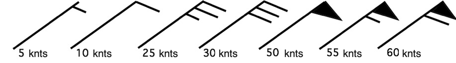
💡 Example: 1 pennant + 2 full barbs + 1 half barb = 50 + 20 + 5 = 75 knots
Precipitation Symbols
| Symbol | Description |
|---|---|
 | Rain (more dots = heavier) |
 | Snow |
 | Drizzle |
 | Showers |
 | Thunderstorm |
 | Fog |
📥 Download: Complete Weather Symbol Guide (PDF) - NOAA
Understanding "Ahead" and "Behind" a Front
These terms refer to front movement, not geographic direction:
| Term | Meaning | Example (Cold Front) |
|---|---|---|
| Ahead of the front | In front of the frontal movement | In the warm air mass |
| Behind the front | After the front has passed | In the cold air mass |
💡 Practical application: If a forecast says "showers behind the cold front," expect precipitation AFTER the front passes through your location.
Common Units
| Measurement | Unit | Conversion |
|---|---|---|
| Pressure | millibars (mb) or hectopascals (hPa) | 1 mb = 1 hPa = 0.0295 inHg |
| Wind speed | knots (kt) | 1 kt = 1.15 mph = 1.85 km/h |
| Temperature | °F (US) or °C (international) | °C = (°F - 32) × 5/9 |
Chart Sources and Frequency
| Source | Coverage | Update Frequency |
|---|---|---|
| NOAA OPC | Atlantic, Pacific, Arctic | Every 6 hours (00, 06, 12, 18 UTC) |
| NOAA WPC | North America | Every 3 hours |
| Met Office | North Atlantic, Europe | Every 6 hours |
| BOM | Southern Hemisphere | Every 6 hours |
Technical References
Official documentation:
- NOAA Unified Surface Analysis Manual (PDF) - Complete 33-page technical reference
- NOAA JetStream - Surface Weather Maps - Official NOAA online tutorial
- WPC Front Codes - Official front symbol reference
Additional learning resources:
- How to read Surface Weather Maps (NOAA JetStream) - Official NOAA guide with illustrations
- Surface Weather Plots (NOAA JetStream) - Station plot details
Permalink
The SHOM Tidal Current Atlas is available for use in routing settings, in addition to GRIB format models (¹).
The Atlas data can be displayed as particles on the chart.
Tap/click on the layer display button, then check “Current Atlases”:
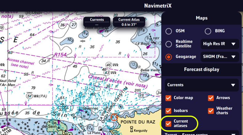
You can overlay this display with a high-resolution GRIB from Ifremer, for example, in order to compare them by dragging the timeline:
Tip: adjust the zoom according to the circumstances for better readability.
–––
(¹) See: How do I calculate a routing?
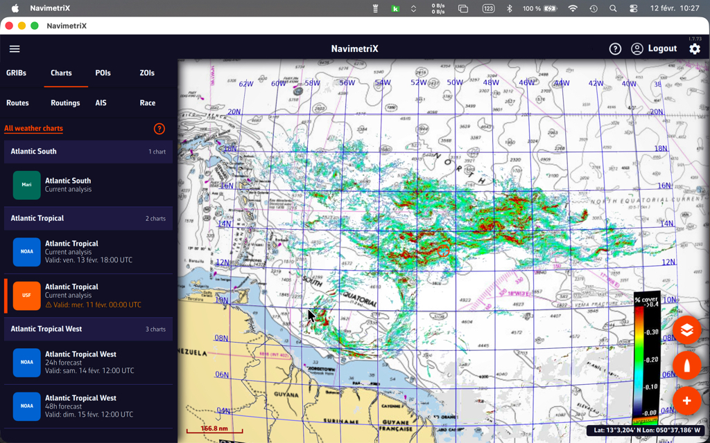
PermalinkNumerous weather surface analysis maps, also known as isobaric or fronts maps, are available in the application to supplement GRIB files and facilitate the interpretation of weather situations and forecasts.
These charts come from various meteorological agencies and are produced by forecasters: NOAA (USA), MetOffice (UK), BOM (Australia), etc. A special chart for observing Sargassum off the coast of the Caribbean is also provided by USF (University of South Florida). All are stored on our own servers and to download from it.

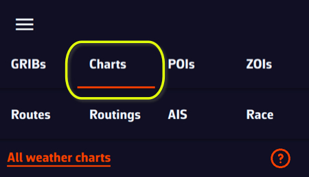
Open the Hamburger menu and select the “Maps” tab.
The Maps menu is dynamic, offering maps available according to the target's location on the world map.
Displaying NOAA weather maps
NOAA maps range from current analysis up to 4-day forecasts, updated every six hours.
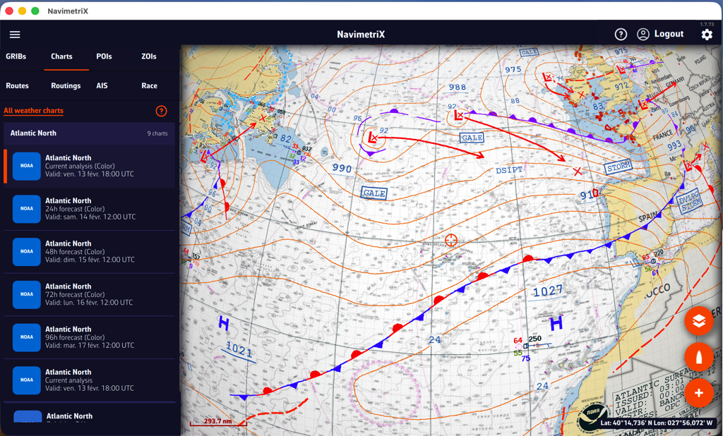
Overlaying NOAA weather maps with GRIBs
Overlaying the NOAA map with the GFS file provides additional insight with the drawing of fronts and specific annotations.
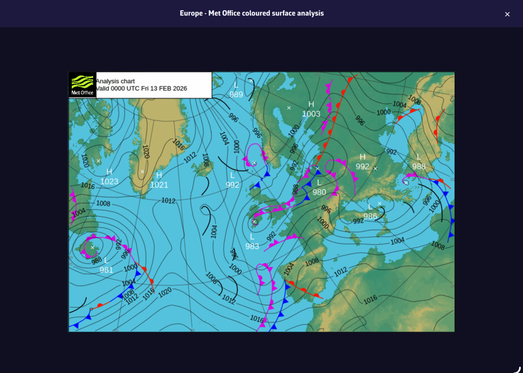
Displaying MetOffice weather maps
MetOffice maps are not in a format that allows them to be overlayed on the nautical chart in 3D. They are therefore displayed in their original format, in color or black and white. They only cover the Northeast Atlantic and Europe. They range from current analysis up to 5-day forecasts.
Sargassum map
Published by the USF, the sargassum density map covers the eastern Caribbean from W38 to W62 and from N20 to the Equator. It is updated daily. It is mainly of interest for crossings to the West Indies.
Satellite images
Three types of satellite images are available, covering the entire world. They are taken from different weather satellites and provide a near real-time view of cloud cover and precipitation.
Tap/Click on the layers button and select the “Realtime satellite” option in the Maps section.
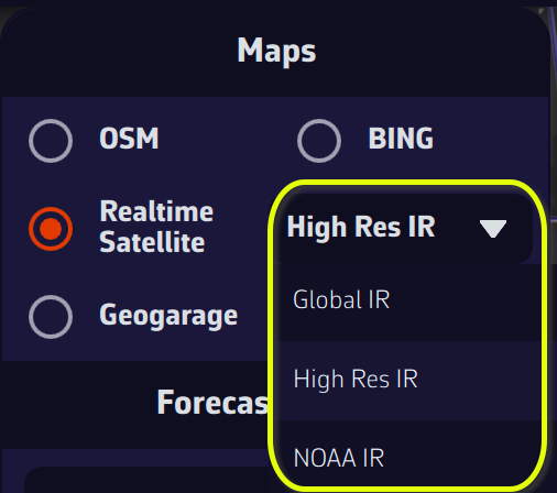
High Res IR, Global IR, and NOAA IR are combinations of infrared images that display cloud cover, and precipitation totals for the first two. By combining a satellite image and an isobaric map, you can obtain an instant view of weather conditions.
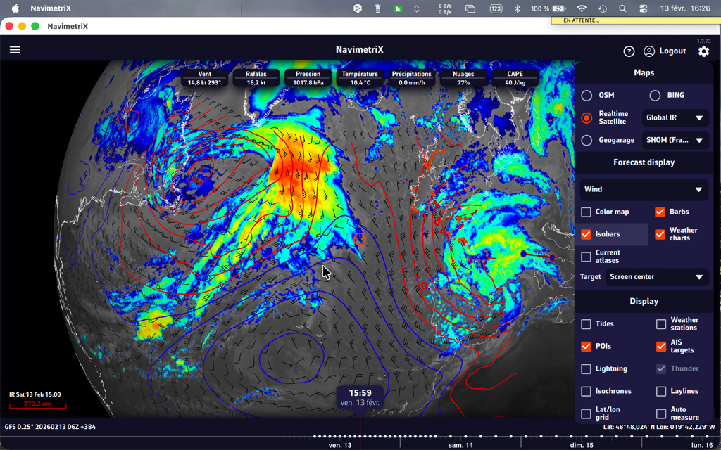
You can also add thunder and lightning displays!
The color coding of precipitation totals on radar images follows the scale below (source: Météo-France) :

For information on interpreting frontology (isobaric) maps, see this FAQ: How to read marine weather maps.
Permalink“In-situ” weather stations provide instant weather readings that allow you to compare this data with weather model forecasts. These stations can be semaphores along the coastline, fixed or floating buoys at sea, accredited ships, airports on land, or weather satellites.
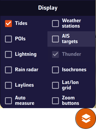
How to display them?
Tap/click on the layers menu and check the “Weather stations” box in the Display section.
The stations are represented by an “arrowhead” symbol that takes the orientation of the “wind direction” data and the colorimetry of the “wind strength.”
Tapping/clicking on a symbol opens a window displaying the characteristics of the station and the most recent data values.
Station types and their info data
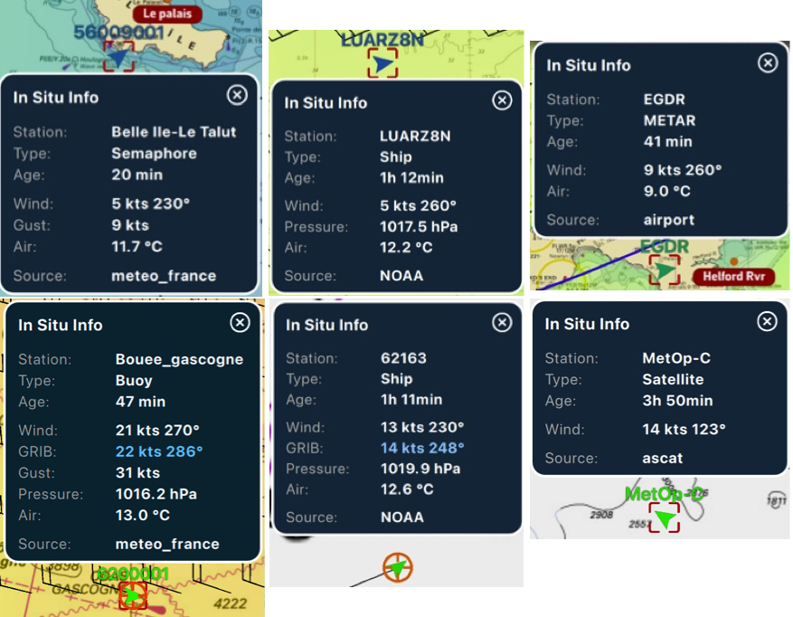
If the time of the information is within the coverage period of the displayed GRIB file, then tapping/clicking in the center of the popup centers the map on the station's coordinates and returns the timeline to the exact time of the station, allowing you to compare the data value and the GRIB file forecast.
Permalink
Set the weather data display in Navimetrix:
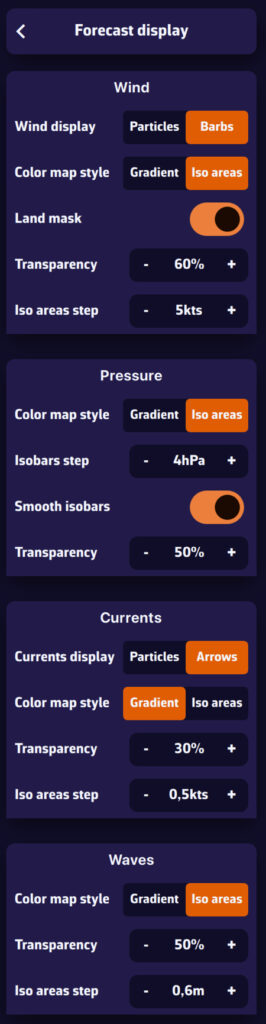
- Open the Settings menu: tap the gear icon in the top right corner.
- Go to the “Forecast display” section: you will see four blocks, each corresponding to a type of weather data:
- Wind
- Pressure
- Currents
- Waves
- Customize the Wind display:
- Barbs: classic display with arrows and small barbs indicating strength.
- Particles: small animated particles representing the flow. Very effective for visualizing the wind, but be careful of battery consumption.
- Color map style: Gradient, continuous color variation, or Iso areas, according to wind intensity.
- Land mask: allows you to easily distinguish land areas.
- Transparency: adjust the visibility of the colored background.
- Step between iso zones: adjust the fineness of the wind ranges displayed.
- Iso areas step: display by ranges (e.g., 5-10 knots, 10-15 knots).
- Customize the pressure display:
- Color map style: Gradient, continuous pressure visualization, or Iso areas (isobars): pressure lines spaced at an interval that you can adjust.
- Isobar step: spacing of isobars in hectoPascals.
- Customize Currents display:
- Classic arrows: direction and strength of currents.
- Animated particles: small animated particles representing the flow. Very effective for visualizing large-scale currents, but be careful of battery drain.
- Color map style: Gradient, continuous current values visualization, or Iso areas (isobars): current values spaced at an interval that you can adjust in knots.
- Customize Waves display:
- Waves are always represented by arrows indicating the direction.
- Color gradient: continuous visualization of wave height.
- Iso areas: wave height spaced at intervals that you can adjust.
Tip: use Particles display mode or Iso areas for better reading of large-scale conditions. For sea navigation, use Barbs and Isobars, which are more accurate and less resource-intensive.
PermalinkYou check the weather forecast before setting sail: southwesterly wind 15 knots, slightly rough seas. Perfect. But how reliable is this forecast? Could it just as easily be 10 knots… or 25? This is exactly the question that an ensemble model answers.
One forecast is good. Thirty-one is better.
A standard weather model such as the GFS produces a single forecast: the best available estimate of the future atmosphere. The problem is that the atmosphere is chaotic—tiny differences in initial conditions can lead to very different outcomes a few days later.
An ensemble model such as NOAA's GEFS (Global Ensemble Forecast System) takes a radically different approach. Instead of running a single simulation, it runs 31 in parallel:
- 1 control run (gec00): the reference simulation, without perturbation
- 30 perturbed members (gep01 up to gep30): each starts from slightly different initial conditions, simulating the natural uncertainty of observations
Result: instead of a single scenario, you get 31 possible futures. If the 31 forecasts converge, confidence is high. If they diverge, it is a clear signal that the situation is uncertain and caution is needed.
The average GEFS model displays wind and pressure with their standard deviation, providing an overview of the uncertainty.
Average and standard deviation: see the uncertainty at a glance
The average GEFS model provides, for each point on the grid, two information:
- The average wind (or pressure) value calculated over the 31 members.
- The spread: the dispersion around this average.
Statistically, there is approximately a 68% chance that the actual value will fall within the range “average ± 1 spread.” In other words, if the average is 15 knots with a 3 knots spread, there is about a 2 in 3 chance that the actual wind will be between 12 and 18 knots. A low spread means a reliable forecast; a high spread means a high degree of uncertainty.
Why it's essential for navigation
While sailing, the weather determines your route, your speed, and your safety. Here's what an ensemble model gives you in concrete terms:
1. Quantifying uncertainty
A classic deterministic model tells you: “15-knot wind.” An ensemble model tells you: “average wind speed of 15 knots, with a spread of 3 knots — so between 12 and 18 knots in 68% of cases.” This information is invaluable for choosing the right sails, planning a backup, or simply deciding whether it's the right time to set sail.
2. Evaluate the reliability of your routing
Your weather routing gives you an optimal route — but this route is calculated based on a single scenario. What happens if the wind shifts 20°? If the low pressure system moves faster? Ensemble routing calculates the optimal route for each of 31 scenarios. If all routes pass through the same location, you can proceed with confidence. If they diverge, caution is advised.
3. Anticipate beyond 5-7 days
The reliability of a classic model declines rapidly after 5-7 days. The ensemble model, on the other hand, remains useful beyond that point, not because it predicts better, but because it shows you how uncertain the forecast is. When the 31 members diverge on D+7, you know it's still too early to decide; that's already very useful information!
GEFS in NavimetriX: easy and accessible
Until now, using an ensemble model was the stuff of professional meteorologists and offshore racing skippers. NavimetriX is changing that by making this data accessible to all sailors:
- Integrated download: the average GEFS model can be downloaded like any other GRIB file, directly from the application (select “Ensemble” from the GRIB request drop-down menu).
- Spread visualization: wind and pressure fields display their dispersion, allowing you to see at a glance where the forecast is reliable and where it is not.
- One-click ensemble routing: NavimetriX automatically downloads and calculates the 31 routes: no need to manipulate files or run scripts.
- Intuitive display: colored “spaghetti” routes and confidence corridor directly on the chart.
The ensemble model is no longer just for experts. It is a tool that helps all sailors make better decisions by transforming uncertainty into visual, clear, and usable information.
PermalinkPOIs and Routes
The term “waypoint” doesn’t exist in NavimetriX. Instead, we use POI (Point Of Interest), a more generic term that can include many elements (targets, anchorages, beacons, race marks, etc.).
Creating a POI
On a tablet or smartphone

Drag the map under the target on the screen, zooming in to position it accurately.
Tap the + icon in the bottom right corner of the screen and select ‘Add POI’ from the menu.
In the creation window that opens, you can:
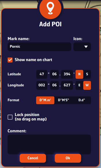
- Enter the name of the point
- Select an icon from the drop-down list
- Choose whether to display the name on the chart
- Enter a specific latitude and longitude manually
- Check that the geodesic format matches
- Lock the POI's position
- Enter a comment about this POI
Tap OK to confirm.
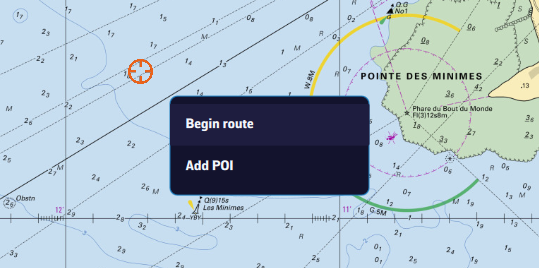
On a Mac or PC
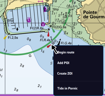
Place the mouse or trackpad pointer on the desired location on the map, without worrying about the target, and right-click. In the popup that appears, select “Add a POI”. The creation window opens as shown here.
Alternatively, you can proceed the same way as on a tablet or smartphone.
Saving
The points are saved in the POI list, located in the left sidebar of the screen, accessible via the ≡ symbol in the top-left toolbar.
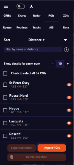
You can show or hide each point individually by tapping the eye icon on the right side of the column.
Adjusting POI display
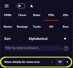
You can adjust the display so that the name and optional icon appear only from a certain zoom level, preventing the map from becoming overloaded if you have many points.
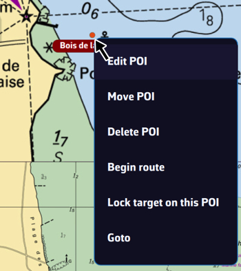
Moving a POI
To move a POI, tap or click on it, select “Move POI” from the menu that opens, then drag it on the map.
On a tablet or smartphone
Move the chart under the target displayed on the screen, zooming in for precise positioning, then tap the + icon in the lower right corner. From the menu, select “Create a route”.
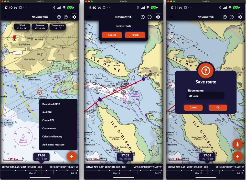
Tap successively to place the desired points. You can drag them with your finger to move them if needed. Zoom in for more precise placement. Once finished, select the “Finish” button at the top of the screen. Enter a name for your route and confirm saving by tapping “OK”.
On a Mac or PC
Click to create successive points, zooming in for better accuracy. You can also drag the points to adjust their position if needed. Click the “Finish” button at the top of the screen. Enter a name for your route and confirm saving by clicking “OK”. Alternatively, you can proceed the same way as on a tablet or smartphone.
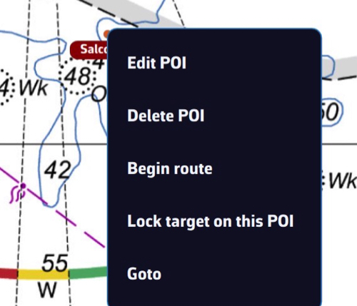
In any case, you can also create a route by tapping or clicking an existing POI (waypoint) and selecting “Begin route” from the popup menu starting from that point.
Saving
Routes are saved in the Routes list, located in the left sidebar of the screen, accessible via the ≡ symbol in the top-left toolbar.
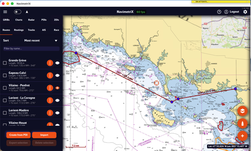
Tap the "eye" icon next to each route to toggle its display on or off. Use the checkboxes to select routes for export or remove.
Reverse / duplicate a route

A "kebab" icon opens a menu with the functions available for the route: Details opens a detailed route log, Reverse, rename, etc.
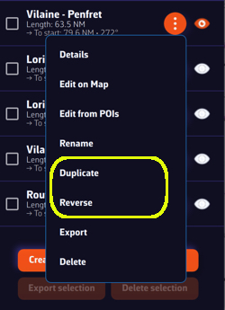
Tap or click, depending on your device, on a POI, and in the menu that appears select “Edit POI” to open the edit window.
You can also move the POI from this menu.
See also: How do I create a POI or waypoint
PermalinkOpen the left sidebar and select the “Routes” section. Display the route on the map by activating the “eye” symbol, then tap or right-click (depending on your device) on any part of the route. In the menu that appears, choose the option “Edit route”.
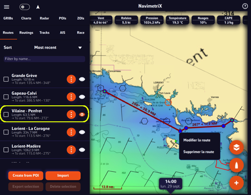
Below, the procedure on a smartphone:
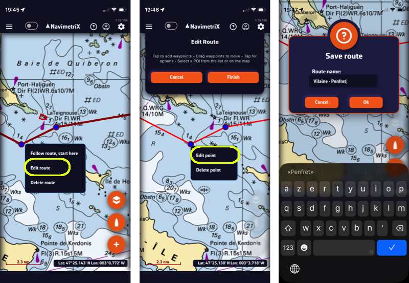
You can then drag points on the map to move them, add new ones by tapping on a segment of the route, and edit or delete any existing route point.
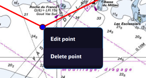
———
See also: How do I create a route?
PermalinkTo start navigation toward a POI (or Waypoint):
💻 On a computer: right-click the waypoint you previously saved, then select Go to. Confirm that you want to navigate to this waypoint.
📱 On a mobile device or tablet: tap the POI, then select Go to and confirm navigation.
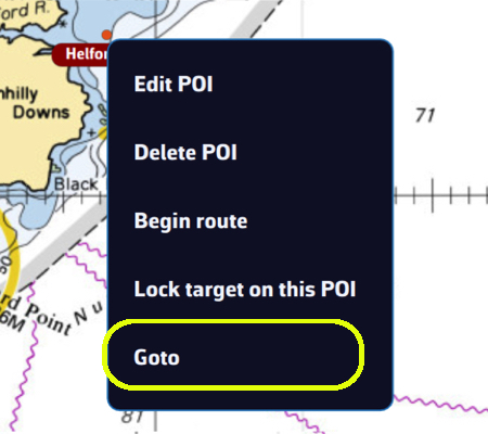
Once the POI is selected, if the boat (the GPS) is at sea, a black dashed line is drawn between your boat and the POI.
To stop navigation, tap or click again on the POI you are navigating to, then choose Stop goto from the menu.
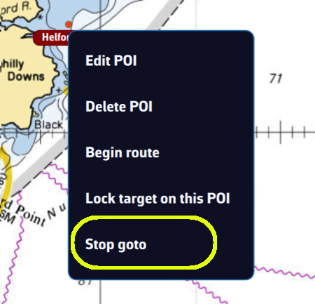
- Check that the option to display POIs is enabled.
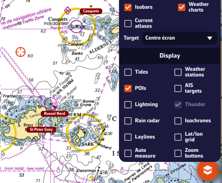
- If POIs only appear when zoomed in too far, lower the zoom level at which they become visible using the option: "Show details for zoom levels over".
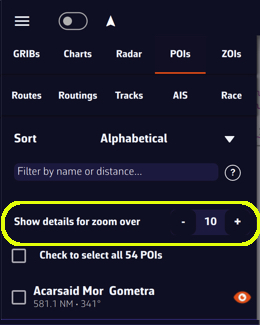
- Edit the route
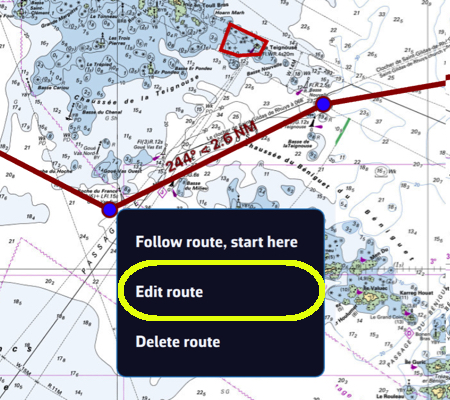
- Edit the waypoint
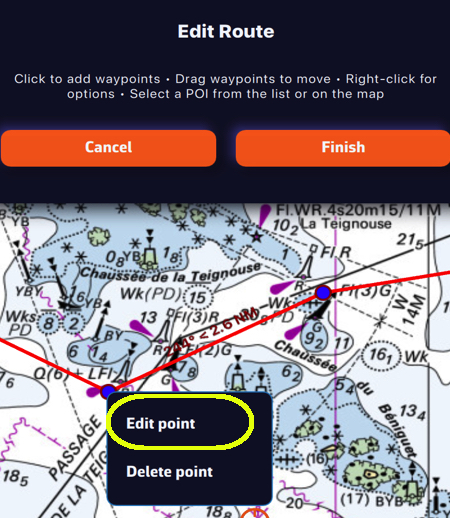
Change the default "Pass by" setting to "Leave to starboard" or "Leave to port"
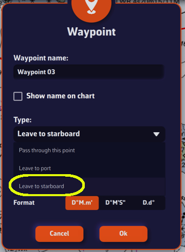
- Green: Leave to starboard
- Red: Leave to port
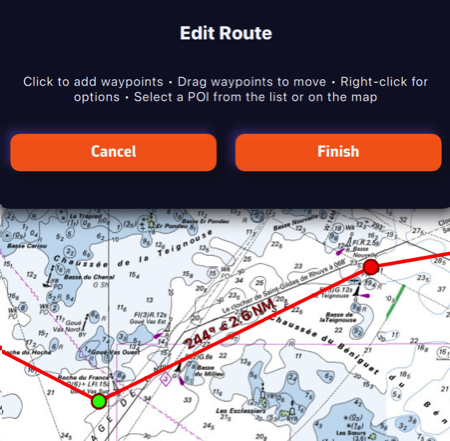
Import POIs
Open "hamburger" menu and select tab POIs :
You can import POIs with extension GPX, KML, and WP (format used by Adrena).
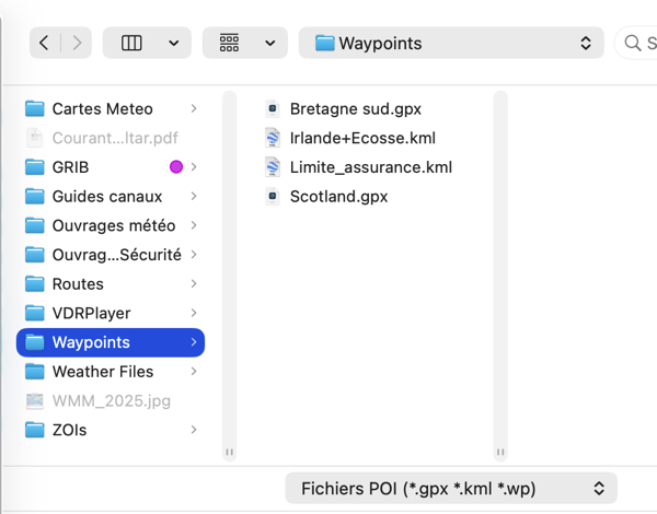
Import routes
Open "hamburger" menu and select the tab Routes:
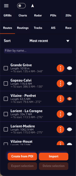
You can import routes with extension GPX, KML, and RT (format used by Adrena).
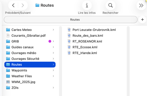
Route tracking allows you to set the boat to automatically navigate through each point on a route. If you control your autopilot by sending it NMEA data (*), it will steer the boat by following the successive legs from one point to the next.
Start route tracking
- Activate "Navigation" mode

- First, display a previously created route.
- Tap or click on the first waypoint from which you want to start tracking.
- Select "Follow route, start here
Activating this feature displays a course deviation corridor, which you can define in Settings > My Boat > Cross-Track:
The cross-track corridor follows all points on the route:
Stop tracking
You can stop tracking or reset the cross-track at any time:
Cross-Track Alarm
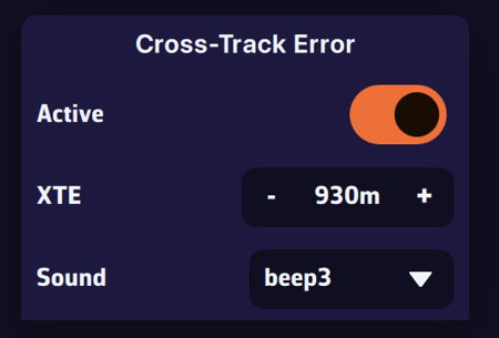
You can enable an alarm if the boat leaves the cross-track corridor.
- Select the Alarms section in the app’s Settings.
- Set the width of the corridor on either side of the direct route.
- Choose a sound from the drop-down menu.
————
(*) See: How to send NMEA data to instruments
PermalinkList of ZOIs
Select the ZOIs tab in the left side drawer.
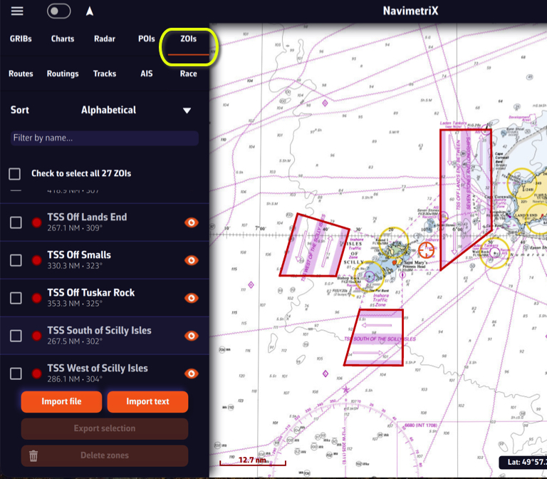
ZOIs are areas to avoid or areas of particular interest. Some are pre-existing in the application, but you can create as many as you need. There are three types:
- No Go Zones: Traffic Separation Systems (TSS), wind farms, protected environmental areas, shallow waters, etc., drawn in red
- Slow Zones: Sargassum fields, speed-restricted areas, areas where sea-state is dangerous, etc., drawn in orange.
- Information Zones: areas of particular interest for navigation, drawn in blue.
You can sort the list alphabetically, by increasing distance, or by date added. You can also search by name.
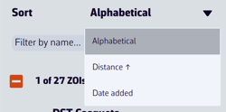
Only no go zones and slow zones are considered by the routing calculation, if they are displayed on the chart. In the left side menu list, you can enable/disable the display of a zone on the chart by tap/click on the eye icon, select one or more zones to export or delete them by checking the box(es). You can also import ZOIs in text format.
Create a ZOI

Modify a ZOI
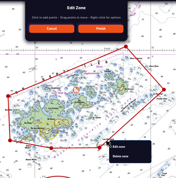
Tap/click on the border of a ZOI to edit/delete it. You can move the borders by selecting the corners, add an intermediate point anywhere on the border to modify it. After selecting the ‘Finish’ button, you can also change the name and type of the zone.
PermalinkRouting
Your boat’s polar determines all routing calculations. It represents your boat’s performance depending on wind speed and angle.
The application supports files in the .pol format (also used by Weather4D, SailGrib, Adrena, and others).
To choose your boat’s polar from the library:
- Go to the “My Boat” tab.
- Click on the selected Polar.
- A dialog opens with three tabs: Library, Imported, or iPolar.
- In the “Library” tab, you’ll find a list of 495 polars for various well-known boats.
Most of these polars come from naval architects or ORC certificates.
To find your polar, you can:
- Scroll through the list.
- Use the search function — for example, type “3600” to find the polar for the Sun Fast 3600.
Once you’ve found your polar, select it and it will be confirmed.
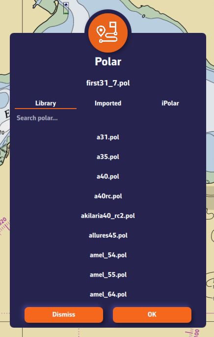
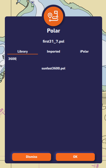
Comment importer une polaire?
The application can import polars in the .pol format.
To import your own polar:
- Go to the “My Boat” tab, then tap the selected Polar.
- Select the “Imported” tab.
- Click on the “Import a Polar” button.
- Choose your .pol polar file saved on your computer or smartphone.
- Once imported, click on the polar to select it.
- The polar is then validated.
Advantage: If you are logged into your NavimetriX account, the imported polar is automatically synchronized across all your devices!
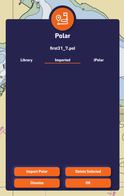
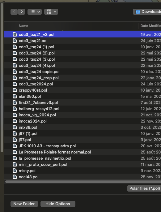
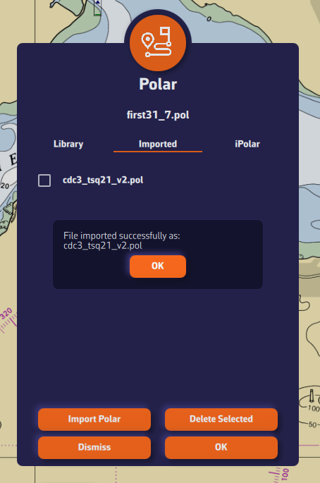
iPolar lets you create a polar in one minute based on your boat’s characteristics:
- Go to the “My Boat” tab, then tap the selected Polar.
- Select the “iPolar” tab, then click “Create”.
- Enter the required information:
- Polar name
- Overall length
- Displacement
- Main sail area
- Jib area
- Optional information:
- Waterline length
- Symmetrical spinnaker area
- Asymmetrical spinnaker area
- Choose your parameters:
- Sailing style: Cruising or Racing
- Polar type: Routing or Performance
- (For most users: Cruising + Routing)
- Click “Calculate my polar”.
- Select your newly created polar.
Note: The iPolar method was developed by KND, experts who work with the America’s Cup, TP52s, and IMOCAs — the best in their field!
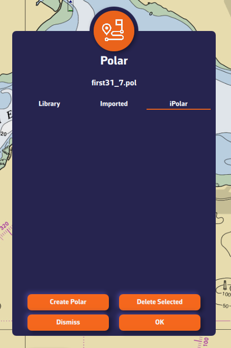
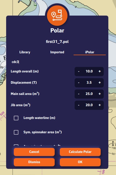
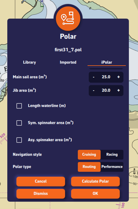
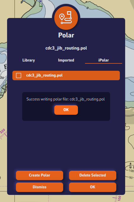
Some polars are formatted as .CSV (Comma Separated Value) files, where the field separator is a comma or semicolon. This format is not supported in NavimetriX, unlike the .POL format where fields are separated by tabs — a format widely used in navigation applications. Therefore, you need to convert your .CSV file to .POL.
With Excel (Windows / macOS)
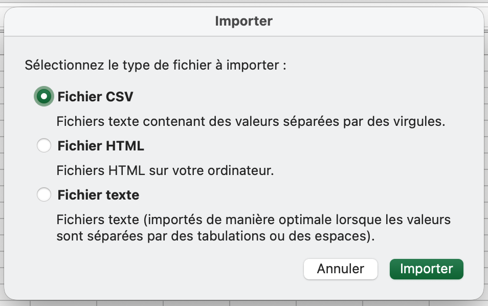
Open a new Excel sheet and select the menu: File > Import.
Choose “CSV File” and then select your polar file from the Finder.
Check the box Delimiters = “Semicolon”, then insert the data into the existing sheet.
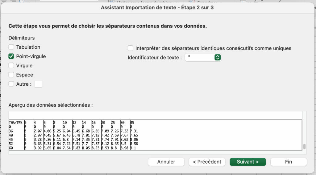
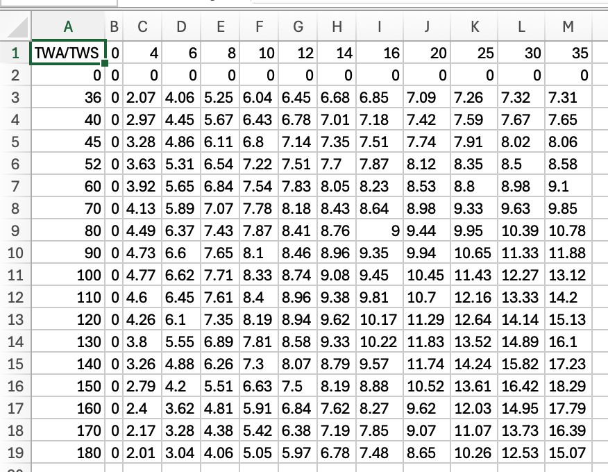
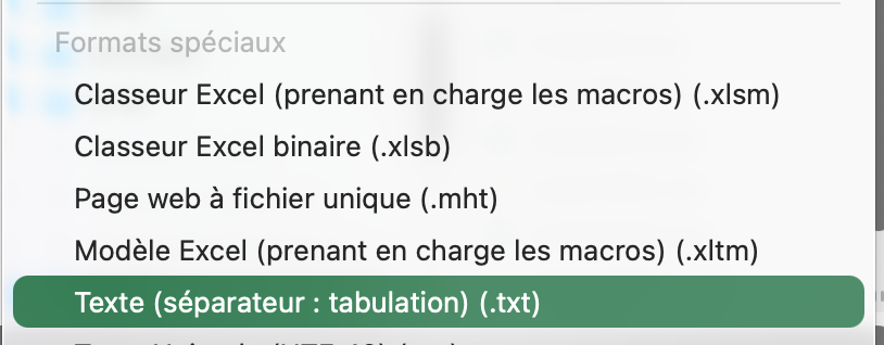
Then save the file in “Text (Tab delimited)” format, which will create a .TXT text file.
Finally, rename the file by replacing the .TXT extension with .POL:
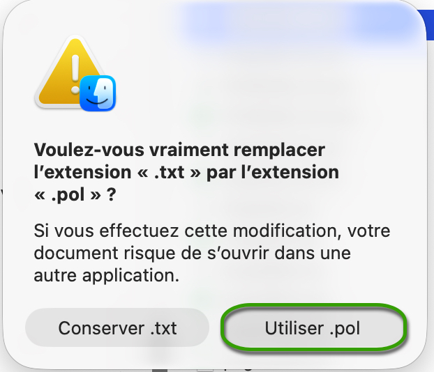
Your polar file is now ready to be imported.
With Numbers (macOS)
Open the .CSV file with Numbers:
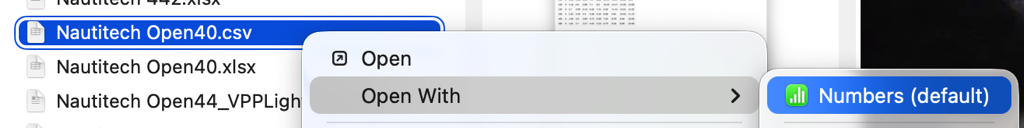
Export the file to TSV:
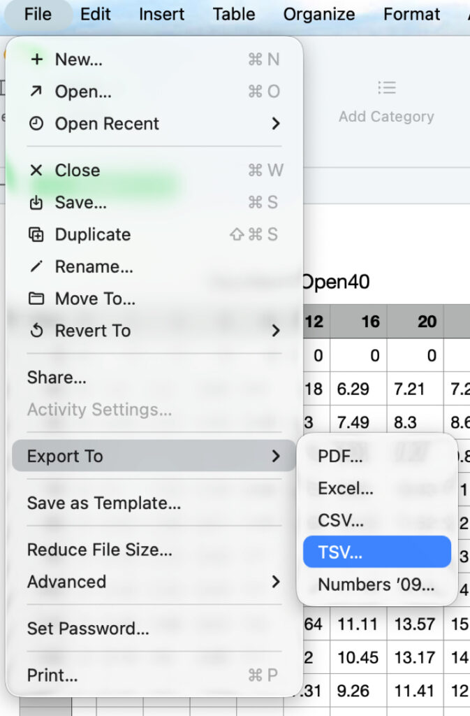
Replace the file .TSV extension to .POL, that's all.
PermalinkTo compute a routing, you must first have:
- Selected your boat’s polar.
- Created a route.
If not yet, see the “Create a route” FAQ. - Downloaded the weather forecasts along the route.
If not yet, see the “Download a GRIB” FAQ.
Once these 3 steps are done, you can compute a routing by pressing the “Compute routing” button.
Remember: a routing is only useful if it’s correctly calibrated and you understand the computed result. Doing a single run and treating it like a train timetable will, at best, lead to disappointment.
We therefore recommend this approach:
- Load the weather, try to understand it and especially the risks,
- always start simple:
- a route that isn’t too complex, so the solver can “breathe”,
- route with wind only,
- no constraints on wind or sea state,
- add currents and waves only if needed,
- for thorough users, study routing stability by varying:
- the wind GRIB speed percentage,
- the polar efficiency percentage,
- run again with another weather model,
- synthesize, understand possible deviations and how you’d react,
- repeat every 12 hours…
1️⃣ Compute a routing

Click the “+” button, then select “Compute a routing”. A screen titled Routing opens.
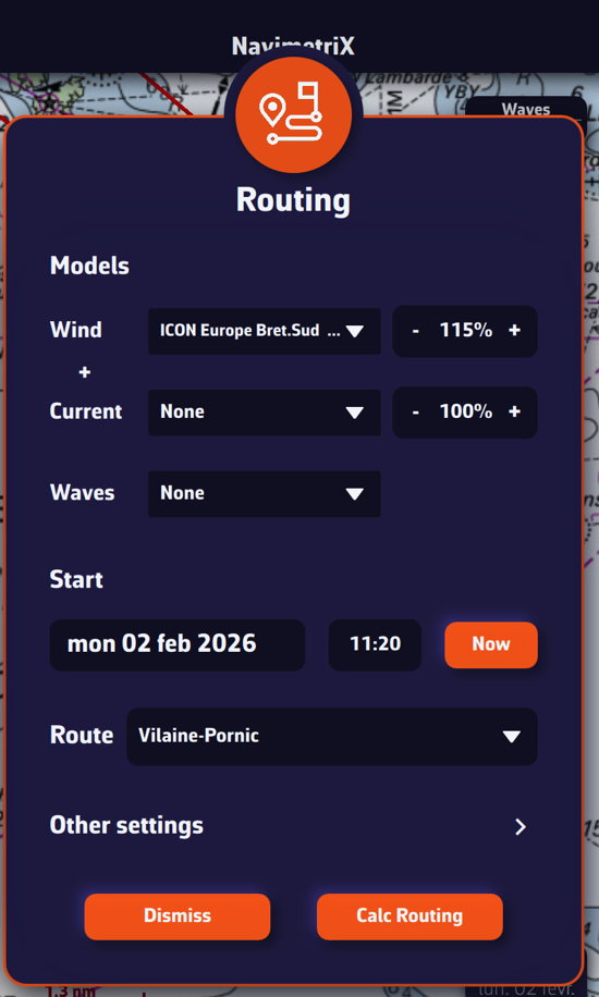
You can choose three forecast models:
- a wind model,
- a current model,
- a wave model.
To begin, select only a wind forecast file.
We recommend setting the wind factor to 115%. This means taking 115% of the wind speed from the GRIB, reflecting that GRIB wind speeds are often lower than reality.
In a second step, following our recommendations, select a current model and a wave model.
2️⃣ Set the departure date and time
Click the date to open the calendar and select your departure date. Click OK.
Click the time to open hour/minute selection, then also validate with OK.
3️⃣ Choose the route
Select the route you just created.
4️⃣ Other settings
These are less frequently modified, but here are the main parameters at a glance.
- Adjusting the boat polar
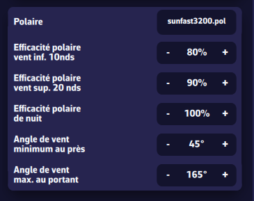
- Polar
See the “Choose your polar” FAQ. - Polar efficiency for winds below 10 kn
Most of the time, speed polars are theoretical and optimistic. If in doubt, set about 80% for a cruising boat. - Polar efficiency for winds above 20 kn
Similarly, polars are often optimistic. If in doubt, set about 90% for a cruising boat.
For wind speeds between 10 and 20 kn, the app linearly interpolates between the two efficiency values to keep the polar “continuous”. - Night-time polar efficiency
This can help if you reduce sail area at night (e.g., take a reef or drop the spinnaker). This multiplicative factor stacks with the two efficiency settings above. Leave 100% to start with. - Minimum upwind true-wind angle
Again, polars are often optimistic. This lets you “trim” the polar to a realistic angle. For example, a Sun Fast 3200’s theoretical polar might show optimal upwind at 36° TWA in 12 kn. In practice it’s more like 40–45°. We suggest 40° with crew, 45° single-handed or cruising. - Maximum downwind angle
For safety: to avoid accidental gybes, don’t sail dead downwind even if the polar suggests it. Set about 165°.
- Routing algorithm
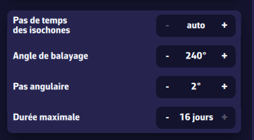
- Isochron time step
Sets the duration of isochrones. We strongly recommend leaving it on Auto. - Sweep angle
Search angle for optimal routes. The faster the boat, the higher you can set it (up to 360°). The default 240° is well-suited to cruising boats and is already higher than the 180° used by most routing software. - Angular step
The angle between each computed route segment.
Leave 2° — that’s usually sufficient. You can go down to 1° for more precision (slower), or 5° on slower devices. - Maximum duration
By default, routing can span the entire GRIB forecast range (up to 16 days). You can limit it (e.g., 3, 5 or 7 days) to compare optimal routes and assess stability. Thanks to a display trick in NavimetriX, this is almost unnecessary.
- Using the engine
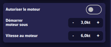
- Allow engine
Check to enable this mode. - Start engine below
Sailing speed below which the engine is started. - Engine speed
Speed once the engine is running.
- Special zones
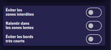
- Avoid restricted zones
Check to make the routing avoid these zones.
These zones can include:- Traffic Separation Schemes (TSS),
- wind farms,
- shoal/shallow areas.
Note: initially, these zones cannot be created or edited. This will come in a future update.
- Constant wind
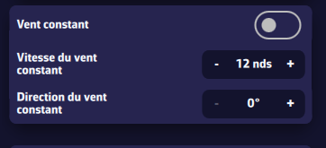
Useful for studying, for example, the effect of current in a bay. It freezes the wind (e.g., as measured at the masthead) to understand the current’s influence on the optimal route.
- Constant wind
Check to enable the mode. - Constant wind speed
Probably the value measured by your anemometer. - Constant wind direction
Probably the value measured by your wind vane.
- Wind and sea-state limits
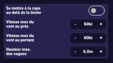
Allows you to constrain the optimal route. Use with care, otherwise the routing may not converge. For example, don’t set a max downwind wind speed of 20 kn for an ocean passage.
- Heave-to beyond the limit
Sets boat speed to 0 kn when a wind or sea-state limit is exceeded.
Most routing software uses a “hard” constraint: you never go through that area once the limit is reached. That can be a bit silly: if a limit is exceeded for 3 hours during a long passage, it’s probably wiser to heave-to for 3 hours than to add hundreds of miles or days to the route. - Maximum wind upwind
Wind speed above which the constraint applies for angles from upwind to beam reach. - Maximum wind downwind
Wind speed above which the constraint applies for angles from beam reach to dead downwind. - Maximum wave height
Maximum “Total sea” height above which the constraint applies.
- Influence of cross sea
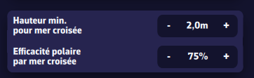
We define a cross sea when the angle between total sea direction and wind sea direction is between 45° and 135°. If the total sea height is high enough, the boat is significantly slowed. You can set the slowdown parameters here.
- Minimum height for a cross sea
Minimum total sea height. - Polar efficiency in cross sea
Multiplicative factor to be combined with the other polar efficiency parameters.
- Reset parameters
It’s easy to get a bit lost among all these settings. The default values were chosen carefully. Press this button to restore them.
Once the routing is computed, the optimal route is shown on the chart together with the isochrone curves. These curves represent the positions that can be reached at successive time intervals from the start point.
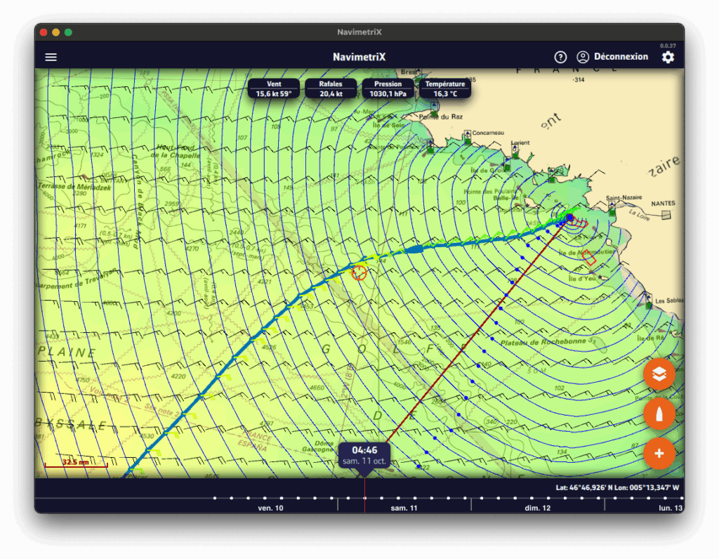
You can move the boat along the route in two ways:
- by dragging the timeline,
- or by tapping directly on the routing at the desired location.
At each intersection between the optimal route and an isochrone, a wind barb is drawn. It indicates the strength and direction of the wind at the moment the boat reaches that position. This is the average wind speed on the isochrone, i.e., the average true wind speed (TWS) used for the routing calculation, which is therefore interpolated geographically and temporally. This is the value found in the routing table. If you are routing with a current, a current arrow will also be drawn according to the same principle as the wind.
Routing list
Open the lists panel and select the Routing tab. This tab lists all computed routings.
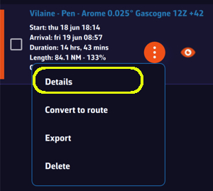
For each routing you’ll see:
- The routing name, shown in a specific color (matching the route color on the chart).
- Departure and arrival times.
- The total duration of the routing.
- The route length and the increase vs. great-circle distance (i.e., the shortest path between start and finish).
- The calculation timestamp.
- An orange "kebab" button that opens a menu of available functions. The "details" function opens the routing table.
- An eye icon to show/hide the routing on the map.
The routing table and its tabs
Click the orange button to open the routing table. It contains four tabs, each presenting a different facet of the computation.
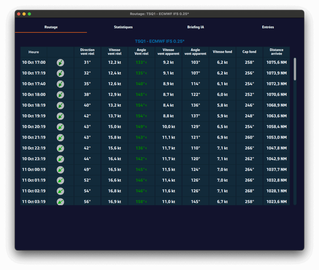
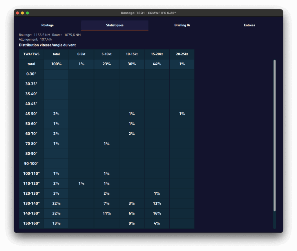
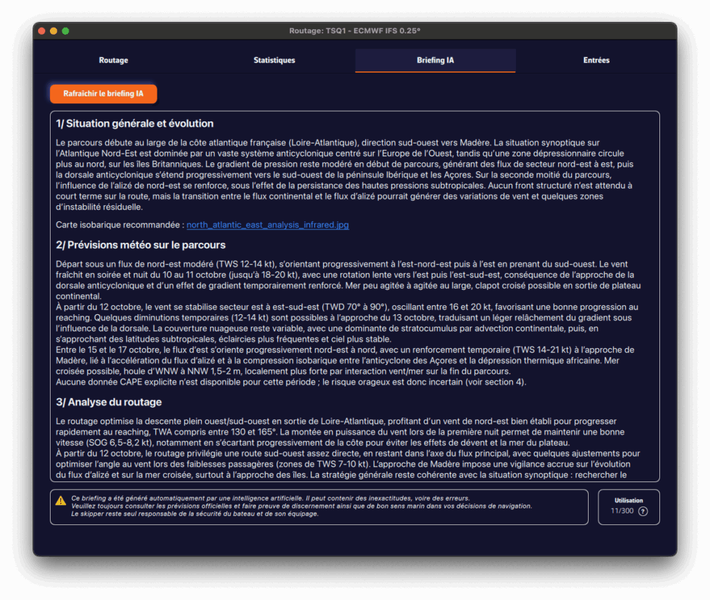
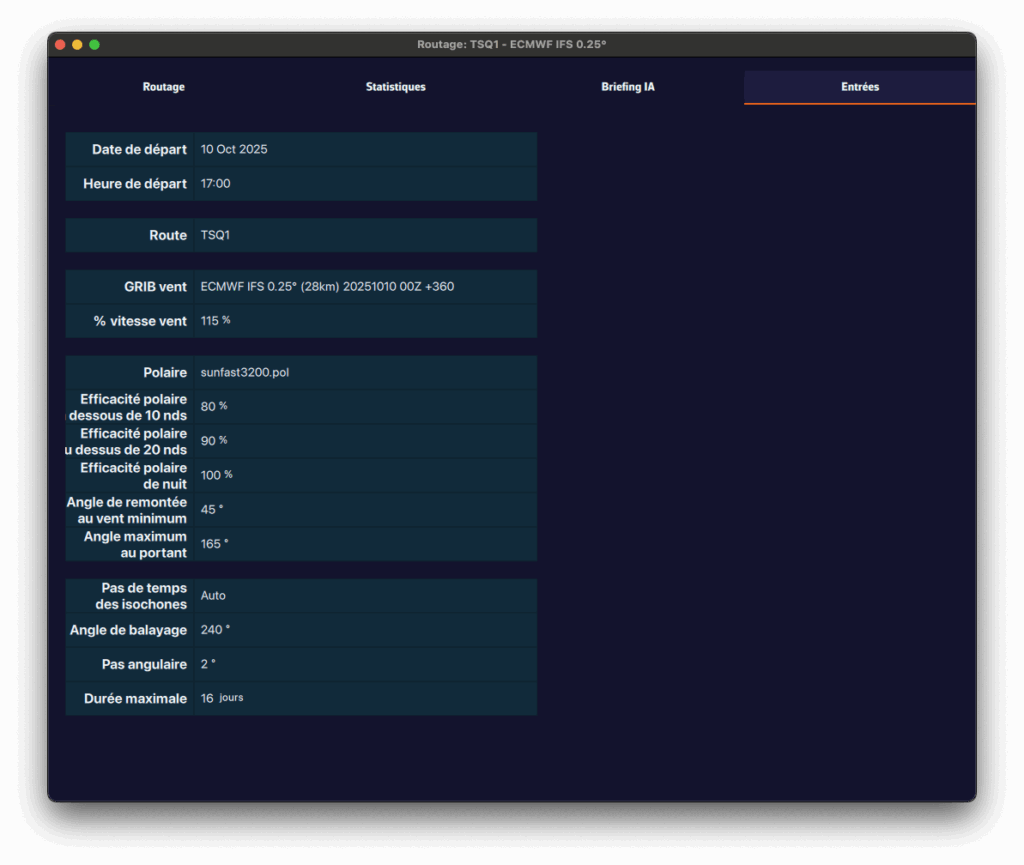
- Routing tab
- Shows, for each isochrone, the boat parameters at that time: speed, wind angle, position, etc.
- Statistics tab
- Displays the distribution of speeds and wind angles encountered during the routing.
- Helps you see whether you’ll sail mostly upwind or downwind, and assess the average wind strength.
- AI Briefing tab
- Automatically generates a weather briefing using our AI.
- When you click Generate AI Briefing, the routing data are sent to our AI server.
- The AI returns a complete briefing with four sections:
- 1. General situation & evolution
- 2. Forecast along the route
- 3. Routing analysis
- 4. Weather risks
- It also includes links to synoptic charts and to the Météo-France bulletin.
- The AI Briefing is a Premium feature. Generation uses AI servers billed per use. Each Premium subscriber has a credit of 300 AI briefings per year, calculated on a rolling 365-day window.
- ⚠️ Warning: this briefing is generated automatically by artificial intelligence. It may contain inaccuracies or errors. Always consult official forecasts and exercise sound judgment and good seamanship in your decisions. The skipper remains solely responsible for the safety of the vessel and crew.
- Input tab
- Summarizes all parameters used for the computation: weather models, coefficients, constraints, and departure settings.
A pivot point is a location you want the routing to pass through.
It’s a very useful way to quickly compare routing options.
For example, in this case we’ll check whether it’s better to pass inside or outside the Traffic Separation Scheme (TSS) off Cape Finisterre — a very common situation when sailing from the French Atlantic coast toward Madeira or the Canary Islands.
To perform a routing with a pivot point, first make sure the isochrones of the desired routing are displayed on the map.
Show or hide isochrones
- Open the Routing list via the hamburger menu (☰).
- Click on the routing whose isochrones you want to display.
- A small orange bar appears to the left of the selected routing: the isochrones are now visible on the map.
- To hide them, click again on the same routing.
Create a routing with a pivot point on a phone
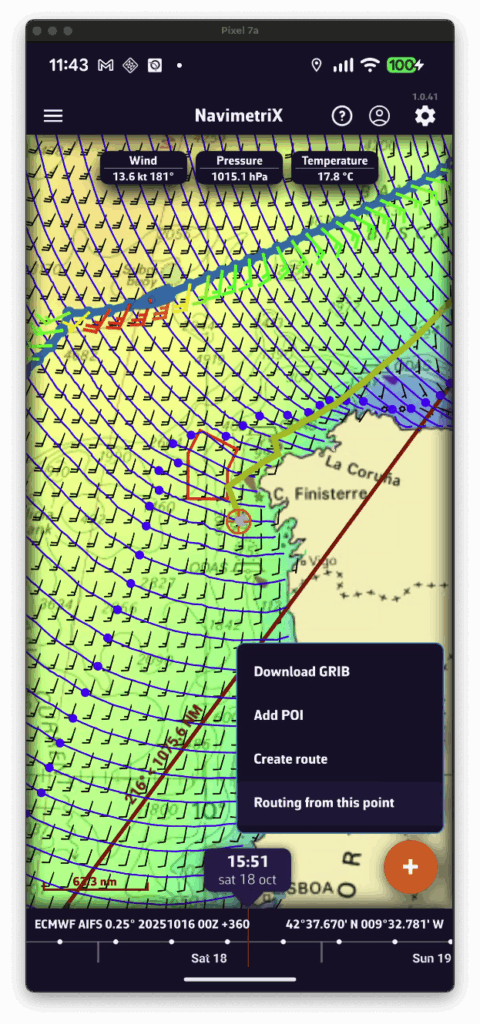
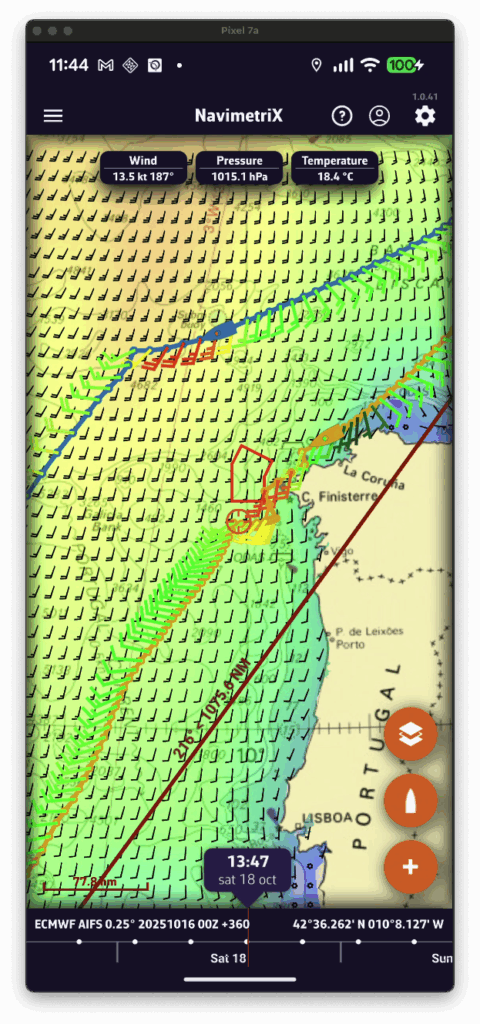
- Display the isochrones of the existing routing.
- Move the map — a yellow route automatically appears toward the center of the screen. It represents the optimal route to the currently selected point on an isochrone.
- If you want to force the route to pass through that point, press the + button and select “Route from this point” in the menu.
- A new routing is then computed starting from the selected pivot point.
Create a routing with a pivot point on a computer
- Display the isochrones of the existing routing.
- Move the mouse — a yellow route automatically appears toward the cursor position. It represents the optimal route to the currently selected point on an isochrone.
- If you want to force the route through that point, right-click on it and choose ”Route from this point” from the context menu.
- A new routing is then computed starting from the selected pivot point.
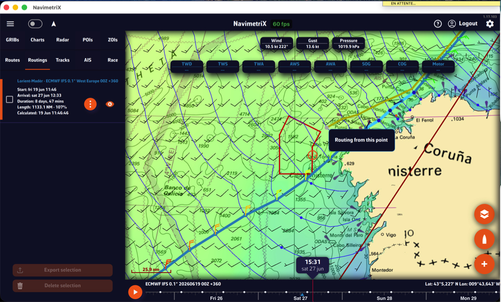
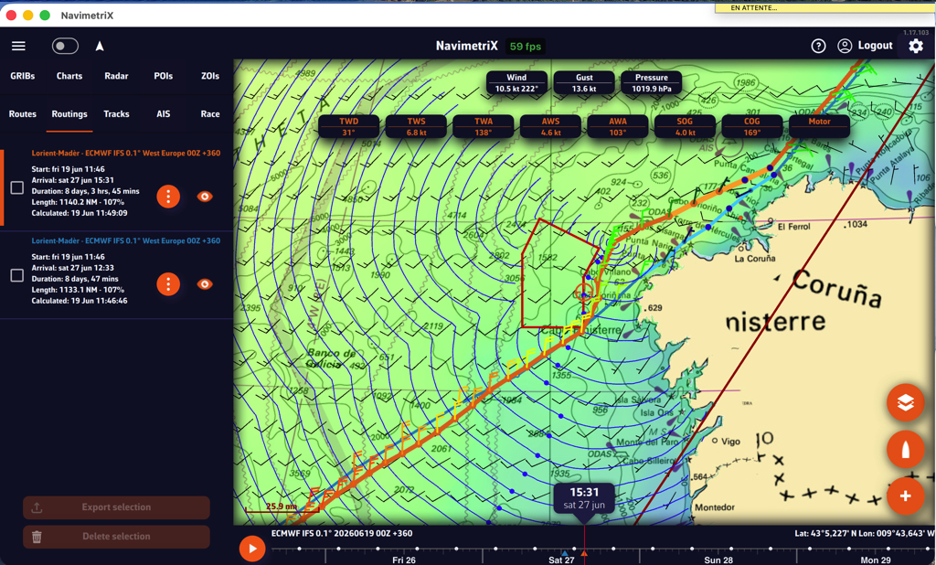
First you have to verify that Isochrones are checked in the Display section of layers menu:
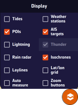
Then simply tap/click on the name of the routing in the sidebar:

When isochrones are displayed, you can use a pivot point.
PermalinkYou can easily convert routing into a route. In the left side panel, from the Routings tab.
Once the routing is complete, open the left side drawer and select the Routings tab.

Select the “kebab” icon and in the menu that opens select “Convert to route”:

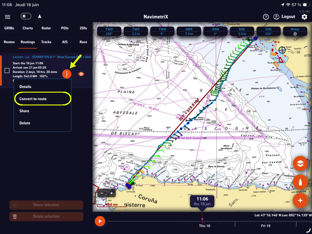
The following window suggests the name of the route derived from the routing, which you can modify, and displays the number of waypoints retained in the routing.
You have two adjustable options: heading tolerance and cross-track error (XTE). Select the “Create route” button and it will be displayed.
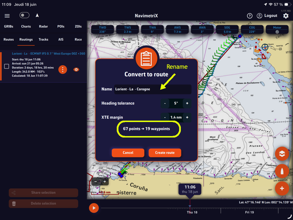
You can hide the display of the routing and the original route.
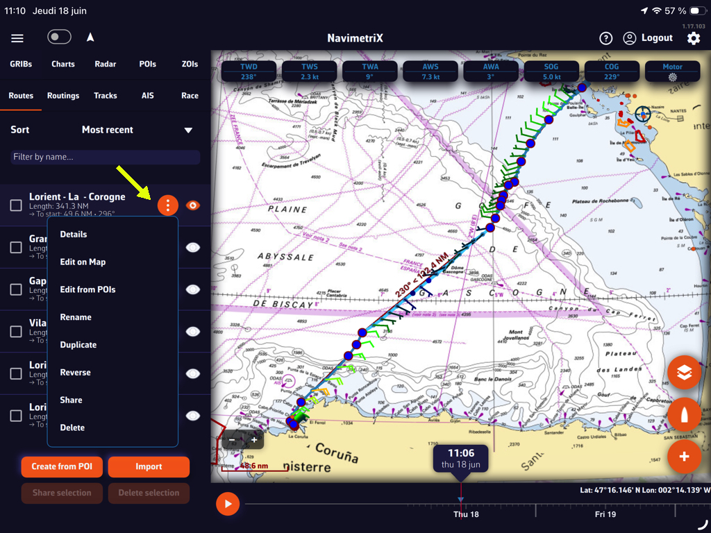
The “kebab” button in front of the created route opens a menu offering several options: route details table, modifications, etc.
PermalinkYou can display simulated navigation data all along the routing.
When isochrones are displayed, data labels in the same colour as the routing boat allow you to track progress along the route. In addition, clicking/tapping on each label displays the data graph from the start to the end of the route.
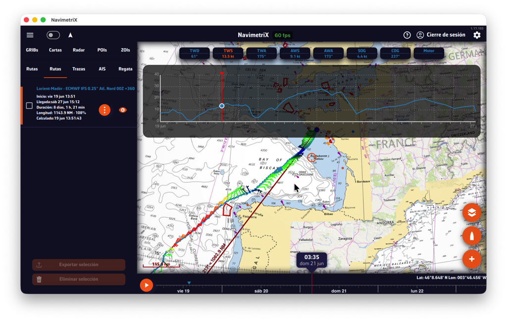
Scroll the boat along the route by dragging the timeline. A "Play" button at the start of the timeline allows automatic timed scrolling.
Tapping the "kebab" button opens an actions menu; the "Details" function opens the automatically generated routing table window.
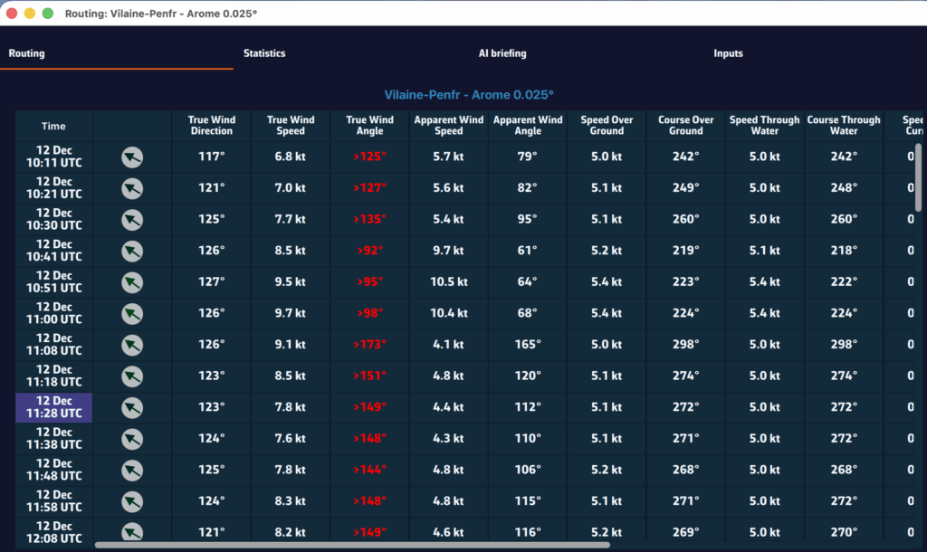
Principle:
An isochronous line is the representation of phenomena known as “isochrones,” i.e., phenomena that have the same time duration.
In maritime routing, isochrones are lines connecting the different distances that can be traveled during a defined period of time, the “step” of the isochrones, in a geographical space — for us, the Earth — based on the polar target speeds of a sailboat.
To connect point A (start) to point B (arrival), the routing will therefore use the speed polar curve and relate it, through iterative calculation, to the average wind data (speed and direction) and current data (speed and direction), taking into account constraints, and multiplying the isochrones along the theoretical route connecting A to B.
How does it work?
The routing algorithm will scan a predetermined search angle, from 180° up to 360°, around the route and proceed with an iteration by calculating a large number of possible routes — this number depends on the search angle/angle step — on the time step defining the isochrones.
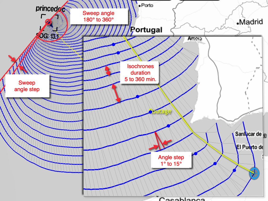
Definitions:
- Sweep angle (or search angle)
From 180° up to 360°, this is the opening angle of the geographical search field in which the isochrones will develop. The default setting is 240°. The chosen opening must take into account the geographical environment of the direct route to the destination point (position of the coastline bordering the route, passage through islands, aso). If the angle is to much open, it may cause divergent routing, too closed the routing may not be able to develop.
- Angle step
Angular steps in the search angle range, from 1° to 15°, default 2°. This is the calculation angle from each point selected on each isochrone. With a search angle of 240° and an angular step of 2°, 120 routes will be calculated from each point selected on each isochrone. The smaller the angle, the more computing power is required.
- Isochrone duration
This is the time between two isochrones. From “auto” by default, up to 360 minutes in 5-minute increments. It must be set according to the distance to be traveled, because the shorter the time step, the greater the accuracy, but the more computing power is required. The “auto” mode lets the program choose the time step based on the length of the leg.
From each isochrone point, the calculation is restarted until the next isochrone and so on until an “optimal path” from the starting point to the destination is obtained.
- Pivot point
On each isochrone, a blue dot shows the shortest distance to the destination. One of these points can be used as a “pivot point” to refine/correct the routing.
Other settings can be used by the developer to fine-tune their routing algorithms for performance optimization.
PermalinkEnsemble routing may seem impressive: 31 route calculations in a single operation with the GEFS 0.5° 30-day model, 51 calculations with the IFS ENS 0.25° 15-day model! In practice, it is as easy as a conventional routing. Here is how to do it, step by step.
Step 1: Download the GEFS model
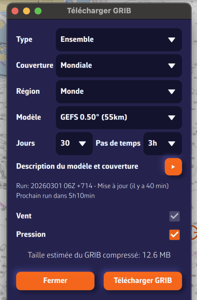
- Open the GRIB file download menu.
- Select:
- Type: Ensemble
- Coverage: Global
- Model GEFS 0.50° (ensemble).
- Choose the desired time period
- Press: Download GRIB
The average GRIB file downloads like any other model; you don't need to do anything special.
The process is the same with ECMWF’s IFS ENS 0.25° model.
Step 2: Configure and launch routing
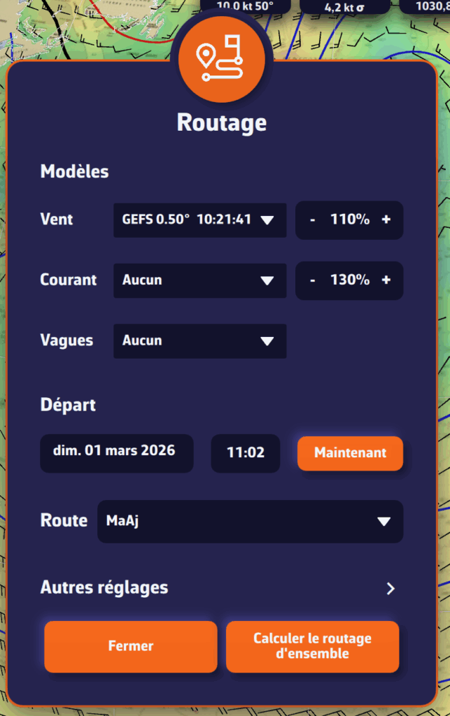
Open the routing window and configure your routing as usual: starting point, destination, ship's polar curve, start date and time...
NavimetriX automatically detects that you are using a GEFS or IFS ENS model based on the model downloaded. The calculation button changes to display "Calculate ensemble routing".
Start routing: NavimetriX handles everything!
- Download the control run (gec00) and calculate its optimal route
- Download and calculate the 30 perturbed members, one by one
- Combine the results and display them on the chart
The whole process is fully automated. Downloading each member takes only a few seconds, and route calculation is very fast. You can follow the progress in real time and see the routes appear one by one on the chart.
Step 3: Track progress
A compact progress panel appears at the bottom right of the screen. It displays in real time:
- The current phase: downloading or calculating
- The current member: "Member 12/30"
- A progress bar for downloads
You can cancel the operation at any time if necessary.
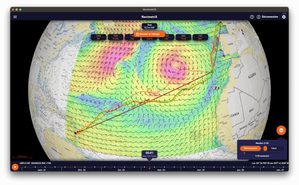
Interpreting the results on the chart
Once the calculation is complete, the chart displays two key elements:
The "spaghetti" routes
Each member is represented by a distinct colored line (the colors are distributed across the entire spectrum to differentiate them clearly). Together, they form a bundle of routes — hence the nickname "spaghetti". At a glance, you can see:
- Closely spaced routes = high confidence. Regardless of the weather scenario, the optimal route passes through the same location.
- Widely spaced routes = high uncertainty. The optimal route depends heavily on actual weather developments.
- Two distinct groups = two possible weather scenarios, with fundamentally different route strategies.
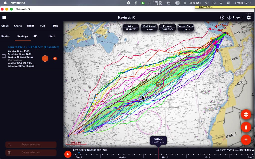
When the "spaghetti" routes converge, outside of waypoints, confidence is high.
The confidence corridor
Overlaid on top, a semi-transparent green corridor represents the range of ±1 standard deviation. Statistically, approximately 68% of routes fall within this corridor. The 20% of members furthest from the mean are automatically excluded from the calculation to prevent extreme scenarios from distorting the visualization.
The corridor gives you an immediate reading:
- Narrow corridor = reliable route, little variability between scenarios
- Wide corridor = high uncertainty, the optimal passage zone is vast
- Corridor gradually widening = confidence decreases over time (typical beyond 4-5 days)
Interpreting statistics
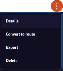
The "Details" function of the "kebab" menu opens the routing table. The Ensemble tab provides a detailed analysis of the 31 scenarios:
- Members who reached the destination: what percentage of the 31 scenarios allowed the destination to be reached? If only 60% reach it, this is a warning sign.
- Distribution of durations: minimum, maximum, average, and median duration. A large min-max spread means that timing is very uncertain.
- Arrival times (ETA): the earliest and latest, to plan your arrival at the port.
- Control run vs. ensemble average: if the control run is significantly faster than the average, the "ideal" forecast is probably optimistic.
- Histogram: visualization of the distribution of durations (or remaining distances if few members reach the finish).
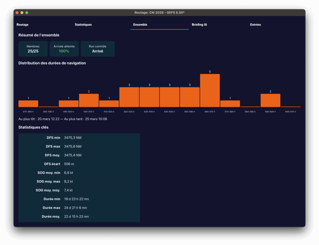
Practical tips
When should you use ensemble routing?
- Crossings lasting more than 72 hours: uncertainty accumulates over time, so ensemble routing makes perfect sense
- Unstable weather conditions: passing fronts, developing low-pressure systems, changing wind patterns
- Go/no-go decision-making: before a departure, ensemble routing helps you objectively assess the level of risk
- Medium- and long-term planning: for a crossing lasting more than 5-7 days, observe the daily evolution of member convergence
Best practices for reading:
- Don't look for "the best route" among the 31 — look for the area of consensus
- Use the time slider to see how the routes diverge over time: the first few days are often close, then the gap widens
- Rerun the ensemble routing when new GEFS data becomes available (every 6 hours) to see if confidence increases or decreases
- Combine with the spread of wind and pressure displayed on the chart to identify areas of high uncertainty

Ensemble routing in NavimetriX transforms an analysis that was traditionally reserved for experts into a visual and intuitive tool. With a single click, you switch from a single forecast to a complete view of the range of possibilities, allowing you to navigate with confidence, even when the weather is not.
___
See also: What is an ensemble weather model and why is it useful for navigation?
PermalinkNavimetriX allows you to select multiple atmospheric models for routing calculations. The principle is to combine multiple resolutions on a given route. This is particularly useful for offshore voyages.
How it works
Multi-GRIB routing works as follows: when several wind GRIB files are added, the application automatically selects the best GRIB for each point and each moment of the calculation, based on three priority criteria:
- The finest resolution first (a GRIB at 0.025° will take priority over a GRIB at 0.25°).
- At equal resolution, the most recent run is preferred.
- At equal resolution and run, the most recently downloaded file is used.
We therefore do not "mix" models, which would not make sense, but "chain" them according to the distance to be covered and the coverage of each model. The multi-GRIB option only works for wind models.
An example:
Let's consider a crossing of the Bay of Biscay, departing from Lorient and arriving in La Coruña. You can use an Arome 0.025° model for the departure, and an ARPEGE Europe 0.1° or ICON Europe 0.0625° model to take over if Arome expires before your arrival. This allows you to calculate a single route instead of two successive routes.
Implementation
After downloading the GRIB files needed to (broadly) cover your sailing area, and activating your route, tap/click on the quick action icon and select "Calculate a route":
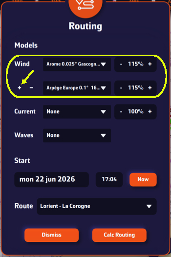
- Select the first "Atmospheric" wind model.
- Tap the small [+] button to select a second wind model with a longer or shorter lifespan than the first choice. The order of the models does not matter, the result will be the same.
- If necessary, select a wave model from "Sea State > Regional".
- If necessary, select a current model.
- Choose your departure date (note: not too far in the future).
- Check that the route is displayed correctly.
- Press the "Calculate Route" button.
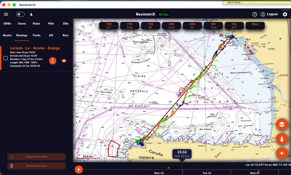
At the end of the Arome model, the routing continues with Arpège.
What is it used for?
The principle is to obtain the best possible resolution at the start of a voyage in order to refine the routing, and only reduce the resolution over the long term.
If we consider a transatlantic crossing, typical use is as follows:
- A high-resolution GRIB (e.g., Arome, Arpège) that covers your departure area with good accuracy but for a limited duration (24-48 hours).
- A low-resolution but long-range GRIB (e.g., GFS, ECMWF IFS) that covers the entire route over several days.
At the start, the routing will use the high-resolution GRIB (because its grid is finer). As soon as the boat leaves the spatial or temporal coverage of this first GRIB, the calculation automatically switches to the second GRIB, which covers the rest of the route.
Notes
1. If only the first GRIB file appears to be used, this may be because both GRIB files cover the same geographical area: in this case, the file with the highest resolution will always take priority across the entire common area.
Make sure the two GRIB files complement each other in terms of geographical and/or temporal coverage. For example, an Arpège Europe for the departure (high resolution, short duration) and a global GFS for the crossing (lower resolution, long range). Routing will then switch automatically from the first to the second once the boat leaves the area covered by Arpège.
2. If two models with the same resolution are used, for example ECMWF IFS 0.25° and GFS 0.25°, the most recent run will take priority when the calculation is launched (for example, GFS 06Z over ECMWF IFS 00Z).
Multi-GRIB is particularly useful when resolutions differ, for example Arpège Europe 0.1° for the coastal area combined with GFS 0.25° for the open sea.
For long distances, you can also use ensemble routing.
Permalink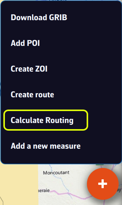
If you have deviated from your initial route, or if you have updated your GRIB files with a new run, you can calculate or recalculate a route underway at any time.
From the quick action button, select “Calculate routing”
With a route already displayed:
- Select the desired GRIB file models,
- Activate the “Start = Now from my position” option,
- Select the next waypoint in the drop-down list of waypoints on your route, according to your progress on the route.
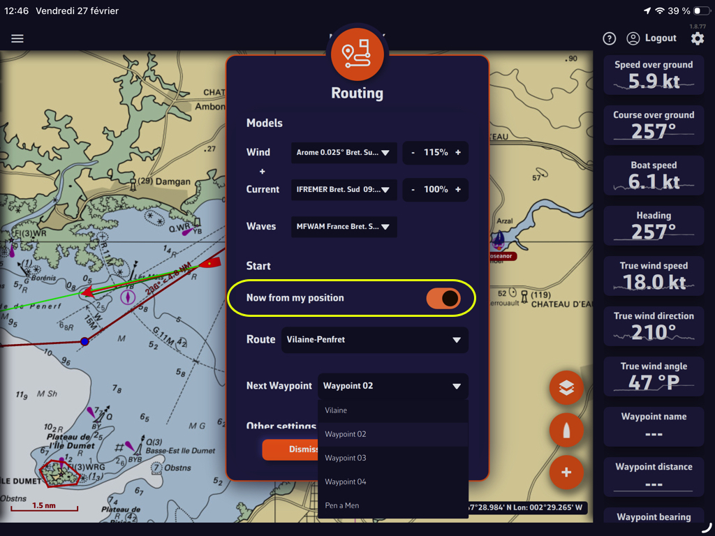
Then simply start the calculation as you would for any other routing.
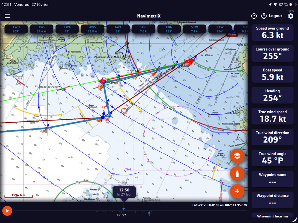
Cartography
Currently, marine charting is provided by the Geogarage platform, where you must create an account and subscribe to one or more services depending on your sailing areas.
An alternative complementary offer, C-Map Discover™X, will be available soon.
Description
The charts offered by Geogarage come from the digital data of numerous international hydrographic offices, such as SHOM, UKHO, NOAA, etc...
About thirty publishers are currently available, offering near-global coverage. These are raster, tiled charts that allow smooth display at different scales depending on the zoom level.
When you subscribe to a hydrographic service through Geogarage, you get access to all the charts published by that hydrographic office.
For example, if you subscribe to SHOM charts (Service Hydrographique et Océanographique de la Marine), you will have access to all SHOM charts.
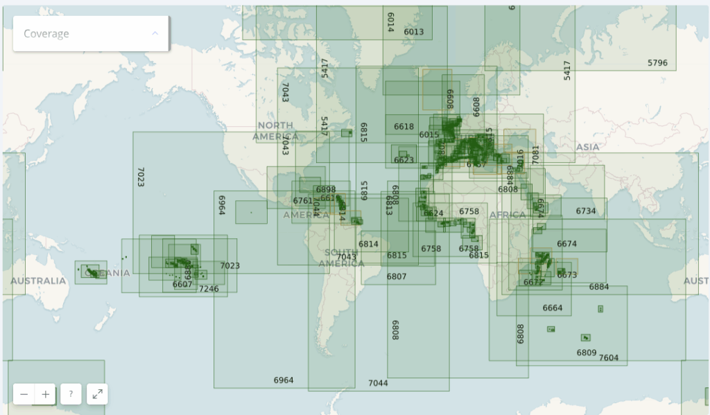
Thus, if you're sailing across the Atlantic from La Rochelle to Fort-de-France, a single SHOM chart subscription is probably enough to cover your entire passage.
Here is an illustration showing the diversity of hydrographic services available in Geogarage:
- the harbour of Toulon by the SHOM (France);
- the Solent by the UKHO (United Kingdom);
- the Kiel region by the BSH (Germany);
- and finally San Francisco Bay by the NOAA (United States).
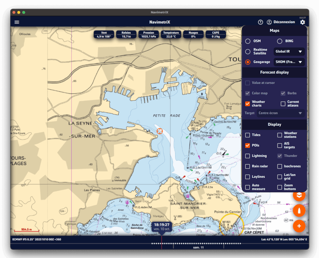
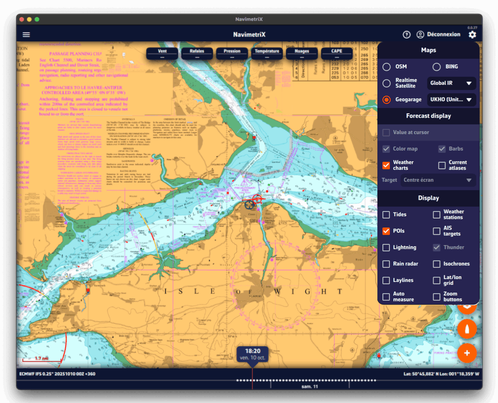
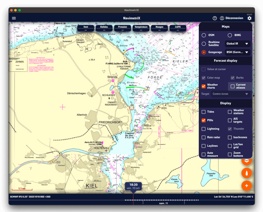
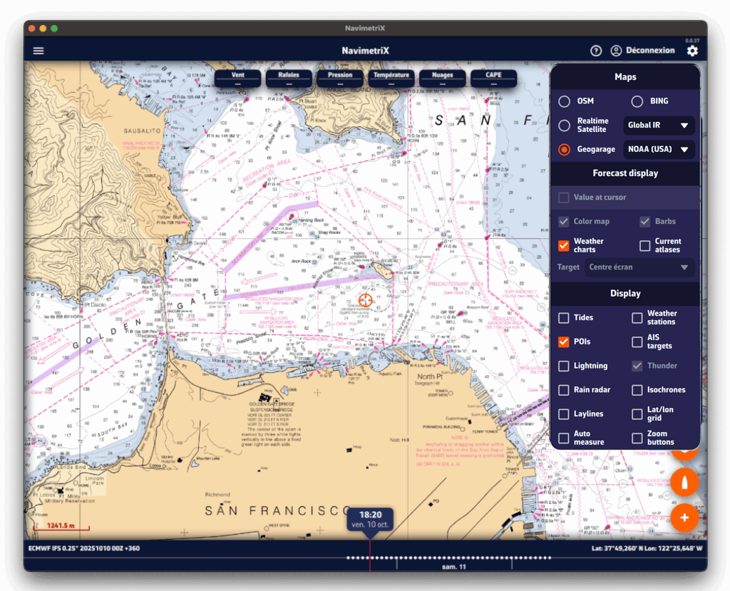
Accessing the subscription page
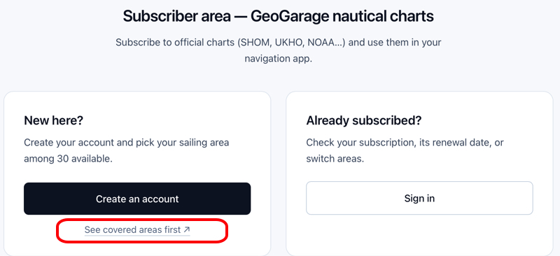
You must first create an account to access the catalog. Note: the credentials you use (email + password) will need to be entered in NavimetriX. Avoid special characters and spaces — a simple combination of digits and upper/lower-case letters is enough.
At this stage, a link already lets you access the areas covered by the catalog directly (red box).
Subscribing to a chart service
Once your account has been created and validated, the offers page is displayed:
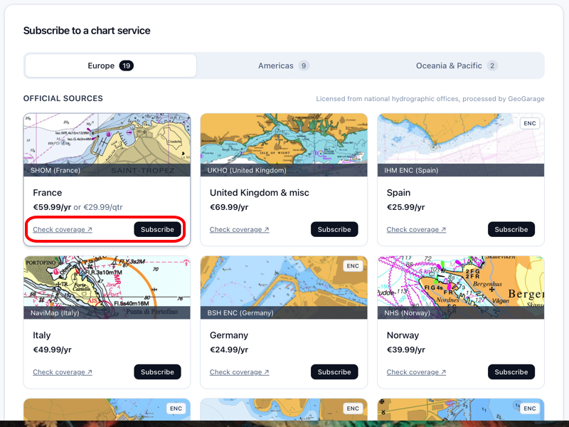
Publishers are presented as thumbnails, grouped by major region: Europe, the Americas, Oceania and the Pacific. You can also check each one's coverage to confirm it includes the level of detail you need.
The "Subscribe" button guides you through the purchase process for your subscription.
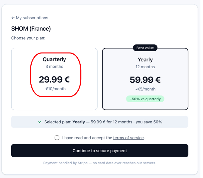
Subscriptions are renewed annually, from one date to the same date the following year, with the sole exception of SHOM, for which Geogarage now offers a 3-month subscription aimed mainly at summer sailors.
Precautions regarding subscriptions
Subscriptions are automatically renewed by Geogarage, by tacit renewal, if:
- You have not indicated that you do not wish to renew,
- Your payment method is still valid.
Geogarage explains the process on their side:
PermalinkIf the subscription is not renewed by its expiry date, the charts — including those saved in the mobile device’s memory — are no longer available for viewing.
A few weeks before the subscription’s expiry date (day J), we send the subscriber a message informing them of the automatic tacit renewal (with a link to opt out if desired), as well as of the expiry of their payment method, if it is no longer valid.
However, the subscription is not cut off on day J itself: several follow-up reminders spaced a few days apart allow a user at sea who cannot check their messages to access this information, or to resolve payment issues with their bank.
However, if no action is taken on the subscriber’s account on our e-commerce site https://accounts.geogarage.com, the subscription is then cut off around day J+15.
Geogarage is an aggregator of official marine charts that brings together vector data from over 30 national hydrographic offices. NavimetriX integrates the entire Geogarage catalog: you can subscribe to any service directly from the app and use official charts on all your devices.
Important: one subscription = a full service, not a region
Unlike Navionics, C-Map or Garmin BlueChart, which sell coverage by geographic region, a Geogarage subscription gives you access to every chart published by a hydrographic office — wherever in the world that office publishes. You pick your subscriptions based on which offices cover your sailing areas, not the other way around.
A few examples:
- SHOM (France): all French charts — mainland and overseas territories (French Antilles, French Polynesia, Réunion, Mayotte, French Guiana, New Caledonia, Saint-Pierre-et-Miquelon, French Southern Territories…). With a single SHOM subscription you get detailed coverage wherever France has dependencies, and global ocean passage charts too.
- NOAA (United States): every chart of US waters — East Coast, West Coast, Gulf of Mexico, Alaska, Hawaii, Puerto Rico, Pacific territories.
- BSH (Germany): all German charts of the North Sea and Baltic.
- UKHO (United Kingdom): all British Admiralty charts covering the United Kingdom and its dependencies (former Commonwealth territories, South Africa, Malta, NGA), and global ocean passage charts too.
For instance: if you sail along the French Atlantic coast and in the French Antilles, a single SHOM subscription covers both areas — no need to buy separate coverage for each archipelago like with other systems. For a long voyage crossing multiple jurisdictions, you combine the subscriptions you need (e.g. SHOM + NOAA to reach the Caribbean from France via the US East Coast).
Hydrographic offices included in the catalog
The Geogarage catalog covers the world's main sailing areas with official charts from:
- Europe: SHOM (France), UKHO (United Kingdom), BSH (Germany), Kystverket (Norway), Sjöfartsverket (Sweden), Geomatikk (Finland), Belgian Hydrographic Service, Danish Geodata Agency, Rijkswaterstaat (Netherlands), Instituto Hidrográfico (Portugal), Instituto Hidrográfico de la Marina (Spain), Croatian Hydrographic Institute, Maltese Maritime Authority…
- Americas: NOAA (United States), Canadian Hydrographic Service, DHN (Brazil), SHN (Argentina), SHOA (Chile), Instituto de Hidrografía (Cuba)…
- Asia–Pacific: JHD (Japan), KHOA (Korea), Maritime New Zealand, Australian Hydrographic Office, Philippine NAMRIA, Taiwan Hydrographic Bureau…
- Africa and Middle East: South African Navy Hydrographic Office, Mozambique, Israel, Oman, regional Persian Gulf services…
Browse the interactive catalog
Select a hydrographic service below to view the exact chart coverage included in its annual subscription:
Annual subscription pricing
Prices vary depending on the hydrographic service and the geographic area covered. You can subscribe to one or several services from NavimetriX. Subscriptions are tied to your account and usable across all your Android, iOS, macOS and Windows devices.
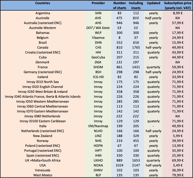
For up-to-date pricing and details, browse the Geogarage interactive catalog above.
Read also
- How can I obtain nautical charts in NavimetriX?
- How do I activate the charts I purchased from Geogarage?
- How do I download charts for offline use?
In the Settings of Navimetrix, under the Geogarage Charts menu, you need to log in by tapping the "Login" button and entering your Geogarage account credentials.
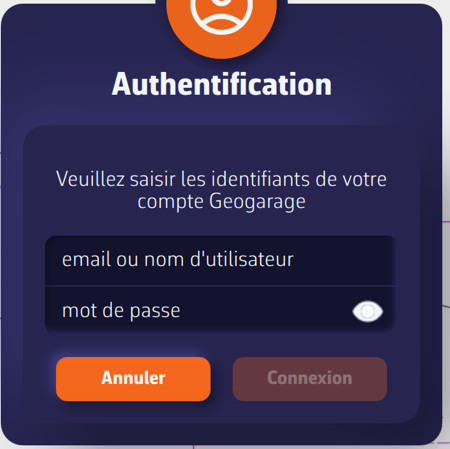
Once connected, select your subscribed chart service (for example UKHO) from the "Layer" dropdown list. The chart display updates instantly while connected to the internet.
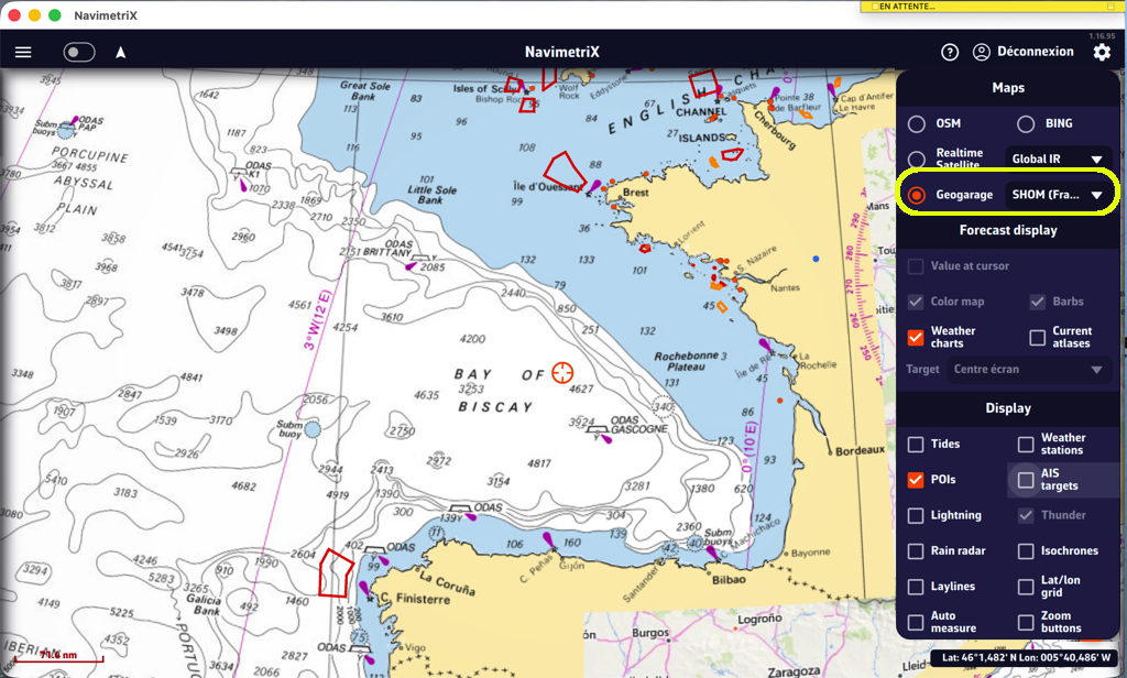
Download
In the Settings of NavimetriX, under the Geogarage Charts section, tap “Add New Zone”, then define the geographical area to download by dragging the green corners of the grey rectangle.
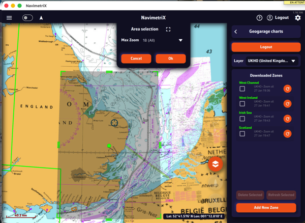
The Area selection dropdown menu offers two zoom-level options for the maximum chart scale:
- 11 (Offshore) — covers a large area containing only small-scale charts (ocean routes, offshore charts).
- 18 (All) — includes all scales up to detailed large-scale charts (ports and anchorages). If the selected area is too large, a warning will appear.
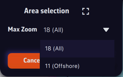
Once confirmed, a countdown shows the preparation and download progress.
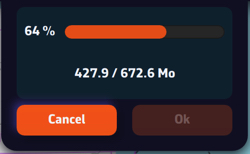
A green frame remains visible so you can add new adjacent download zones without overlap using the “Add a new area” button. Only downloaded charts are available for offline use.
Updating downloaded charts
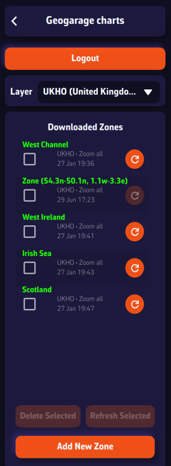
The downloaded chart zones are listed by publisher in the Geogarage Charts drawer. A checkbox allows you to select them for the Delete or Refresh functions.
Whenever a chart update is published by the provider, the dimmed refresh icon becomes active so you can update your zones individually, or collectively by checking the boxes and using the “Refresh Selected” button.
PermalinkIn order to rename a chart area, you have to do a long click/tap on its name. This will bring up the keyboard, allowing you to change the name:
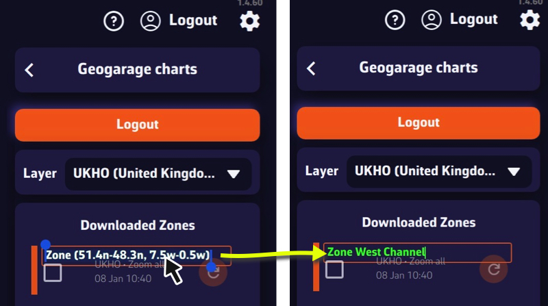
Please note that unlike GRIBs, downloaded charts are not synchronized, and therefore neither is the name.
PermalinkNavigation
Display GPS data from your phone
While sailing, if you want to display your phone’s GPS data, open the app settings (gear icon in the top-right corner).
Go to the GPS & NMEA menu and make sure the GPS source is set to Internal.
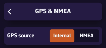
Exit this menu, then open Instruments. Check the Visible box to show the instruments, and make sure the selected layout is GPS View.
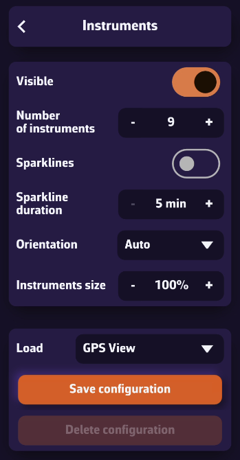
Once your phone receives a GPS signal, the time of the last position, your speed over ground (SOG), and your course over ground (COG) will be displayed in the instrument bar.
You can scroll through the parameters to view your coordinates and POI data if you’ve selected a waypoint using the Go to function.
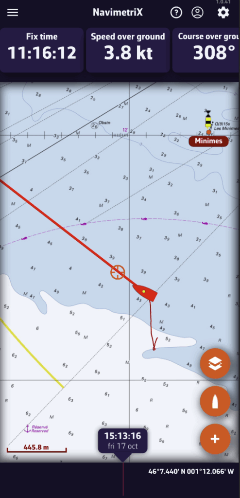
On phones, the default display is horizontal.
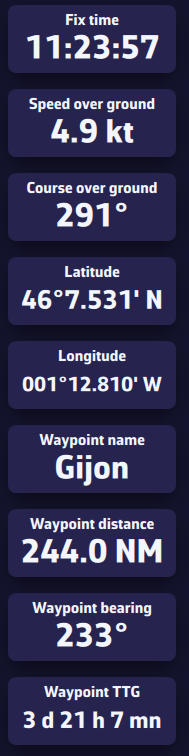
On tablets or computers, the layout automatically adjusts to a vertical view.
PermalinkUSB-connected GPS devices, a.k.a GPS Mouse, are supported by NavimetriX for Mac and PC compatible computers. It provides position to the system's location service.
Prerequisites
A driver matching the connected device must be installed in the operating system beforehand. These are usually Prolific or FTDI drivers, depending on the type of device connected.
Implementation
Open Settings by tapping on the gear icon, then select GPS & NMEA.
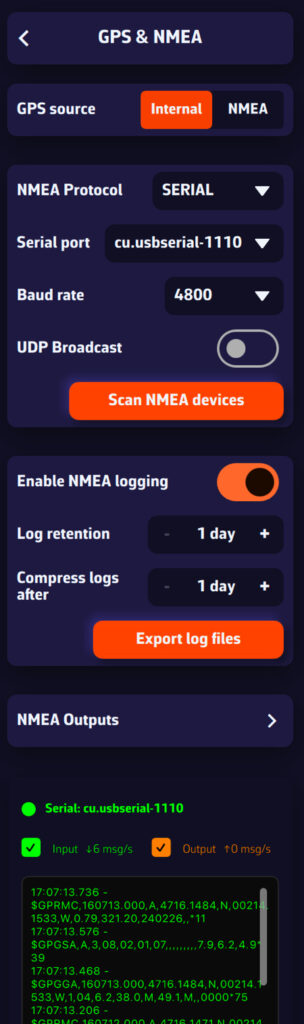
Select:
- GPS Source = Internal
- NMEA Protocol = SERIAL
- Serial Port = scroll down the menu and select the appropriate port (normally the default port is displayed).
- Baud rate = 4800 Bps by default.
Data stream should scroll in the lower window.
Tip: if the serial port does not work, open the drop-down menu and check if another port is available. If no port is available, the driver is probably not the right one.
PermalinkCustomizing the Instrument Panel
To change the displayed instruments, open the right panel using the gear button at the top right of the screen, then select Instruments.
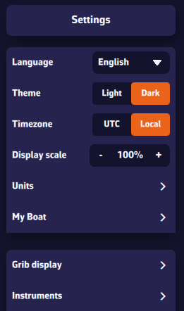
You will see several settings:
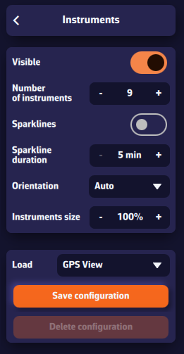
- Visible — Show or hide the entire instrument bar.
- Number of instruments — You can display between 2 and 15 instruments at the same time.
- Mini charts — When enabled, a small chart appears under each instrument showing how the value has evolved over the last 5–20 minutes.
- Orientation — Choose between vertical or horizontal layout, or leave it on automatic (it adapts to your screen width).
- Scrolling — In horizontal mode (especially on phones), you can scroll the instrument bar to the right to see more instruments.
- Instrument size — Adjust the size as you prefer. Increasing it makes the values easier to read — even without glasses!
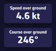
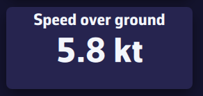
Personalizing your setup
On a computer, right-click an instrument. On a mobile device, perform a long tap.
A list of parameters appears — select the one you want to assign to that instrument. We advice to proceed from the first instrument down to the last one for a more easy way.
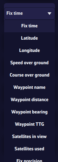
Saving a configuration
To save a configuration, press the Save Configuration button, enter a name, and confirm to save it. This allows you to switch between different configurations according to your needs by selecting their name from the drop-down list.
Saved configurations are specific to each device — they are not synchronized between your phone and your computer, ensuring optimized layouts for each screen. The order remains the same in vertical or horizontal display.
Receiving NMEA Data
To receive NMEA data from your onboard instruments:
- First, make sure you are connected to the Wi-Fi network of your NMEA server or repeater (MiniPlex, NKE Wi-Fi box, etc.).
- Open the Settings panel at the top right (gear icon).
- Select the GPS & NMEA menu.
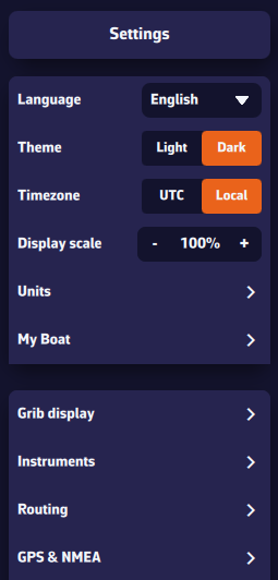
GPS Source
The first line corresponds to the GPS source. If you want to receive GPS data through an NMEA stream, select NMEA.
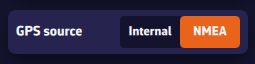
NMEA Source
- NMEA Protocol dropdown menu — preferably UDP, or TCP if required. DEMO — only for demo mode with AIS simulation
- Server IP Address — the IP of your NMEA server or repeater (MiniPlex, NKE Wi-Fi box, etc.).
- Server Port — the port number used by your NMEA source.
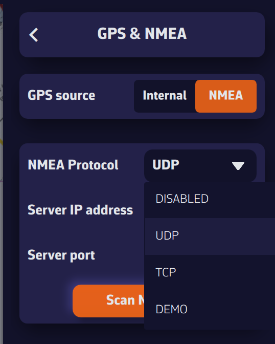
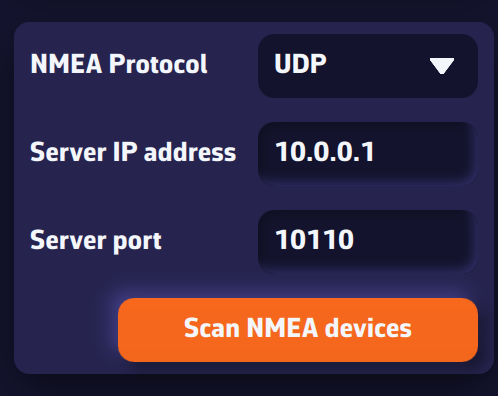
If you don’t know these values, press Scan for NMEA Streams. The scan will automatically search for known configurations. When a stream is detected, NavimetriX will offer to apply the parameters automatically (protocol, IP, port). Select Yes and close the scanner — your NMEA source is now active!
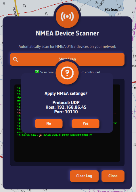
Once connected, NMEA data appears in green in the log window at the bottom of the panel.
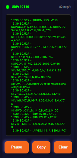
If no stream is found, enter your NMEA system parameters manually. We recommend using the UDP protocol for maximum flexibility.
NMEA Log
The last section lets you enable NMEA logging. When enabled, all received NMEA sentences are recorded. You can set a retention period (for example, 8 days) and specify when the logs should be compressed. Uncompressed daily files can be large (around 60 MB), but once compressed, they are only about 10% of their original size.
The Export Logs button allows you to save these files for analysis or replay with external tools such as VDR Player.
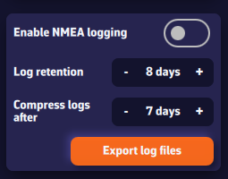
Note: A built-in feature to replay NMEA logs will be added in a future version of the app.
Prerequisite: make sure your NMEA stream is properly configured and that you are receiving AIS sentences (they start with AIVDM).
Note: AIS targets are only visible when "Navigation" mode is enabled.
Enable AIS target display
Open the Settings panel (gear icon, top right).
- Select AIS.
- Enable Show AIS targets.
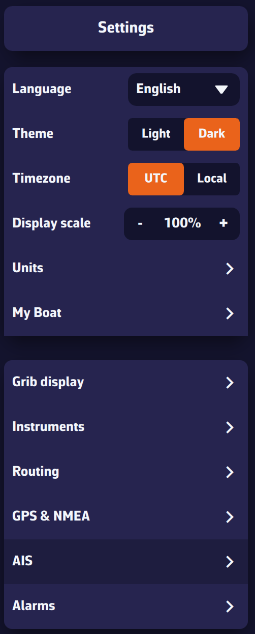
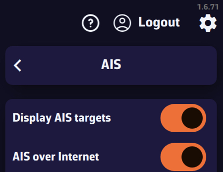
Display settings
- Name & speed: show/hide target name and speed (global setting).
Tip: turn off near the coast when many targets are visible; turn on offshore when few targets are visible. - Remove lost targets after: time before a target disappears without a received sentence (e.g., 15 min). The target fades out: 100% visibility after a recent sentence down to 0% at the timeout.
- COG vector length: course-over-ground vector length, from 0 to 60 minutes.
- Show target track: global option to display tracks for selected targets or for all targets.
Tip: “selected” near the coast (many targets), “all” offshore (few targets). - Track length: Tip: short near the coast (busy areas), long offshore (few targets).
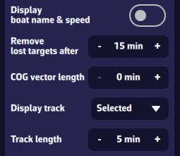
Proximity alarms
- CPA (Closest Point of Approach): minimum distance at closest approach.
- TCPA (Time to CPA): time remaining until CPA.
- Triggering: the alarm triggers when both conditions (CPA and TCPA) are met.
- CPA lines: option to show/hide CPA lines on the chart.
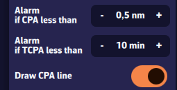

Hide Class B AIS targets
You can hide Class B AIS targets (small recreational boats) to show only Class A (cargo, ferries, etc.)—useful at crowded race starts.
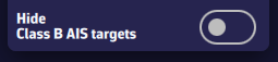
Chart interactions
- Icons: green by default. Chevron for Class B, triangle for Class A. Targets in alarm are red.
- Short tap/click on a target: select it and show its track, name (or MMSI if unknown), and average speed over 5 and 20 minutes.
- Long press: detailed panel with:
- MMSI and Name
- Navigation status: at anchor, restricted maneuverability, fishing, …
- Position: latitude & longitude
- SOG: instant speed over ground; averages over 5 and 20 minutes
- HDG: heading
- RNG/BRG: range and bearing
- CPA/TCPA
- Crossing: ahead of/behind the target (very useful underway)
- Position age
- Static info if available: callsign, type, length, beam, destination
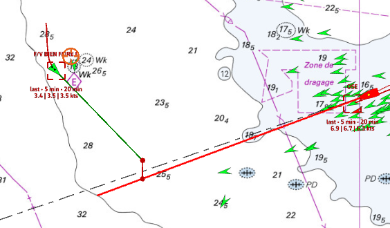
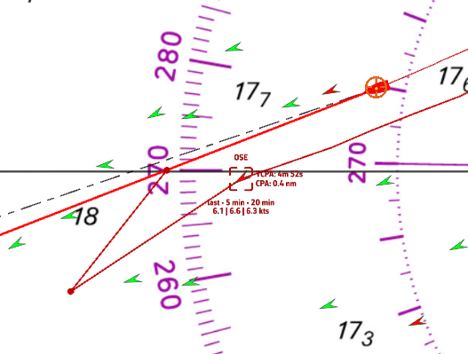
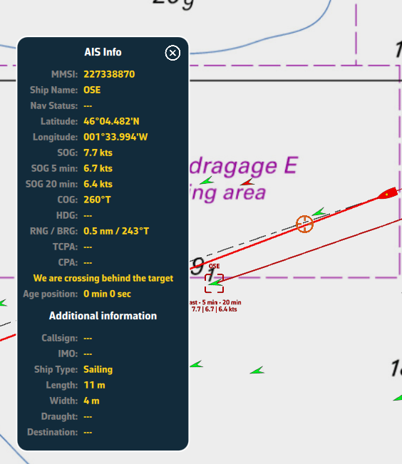
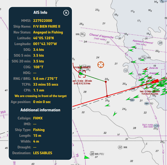
AIS target list
Open the hamburger menu (☰ top left) and choose the AIS tab to display the target list.
For each AIS vessel, the following information is available:
- MMSI and vessel name
- Instant speed
- Speed over ground (5 min)
- Speed over ground (20 min)
- Heading (COG/HDG)
- Range to the vessel
- Bearing
- CPA – Closest Point of Approach
- TCPA – Time to Closest Point of Approach
- At the left of each row, a small color rectangle shows the target state: green if normal, red if an alarm is active.
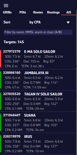
Sort and filter the AIS target list
To quickly find a vessel, you can sort and filter the AIS target list.
- Sort by:
- MMSI
- Name
- CPA and TCPA
- Range
- Instant speed
- 5-min speed, 20-min speed (popular in racing to monitor competitors)
- Filter by:
- Name (e.g., type “CHA” to find “Cœur de Chauffe”, “Alyocha”, etc.)
- Class: type A (Class A) or B (Class B)
- Status: type “Alarme” or “Alarm” to show only targets with a collision alarm
- Click/Tap a vessel:
- the map recenters on the vessel and the target is automatically selected.
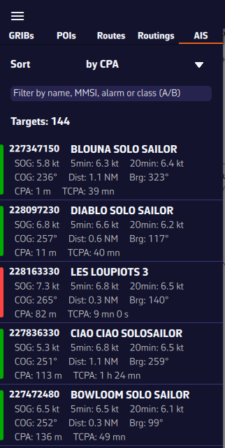
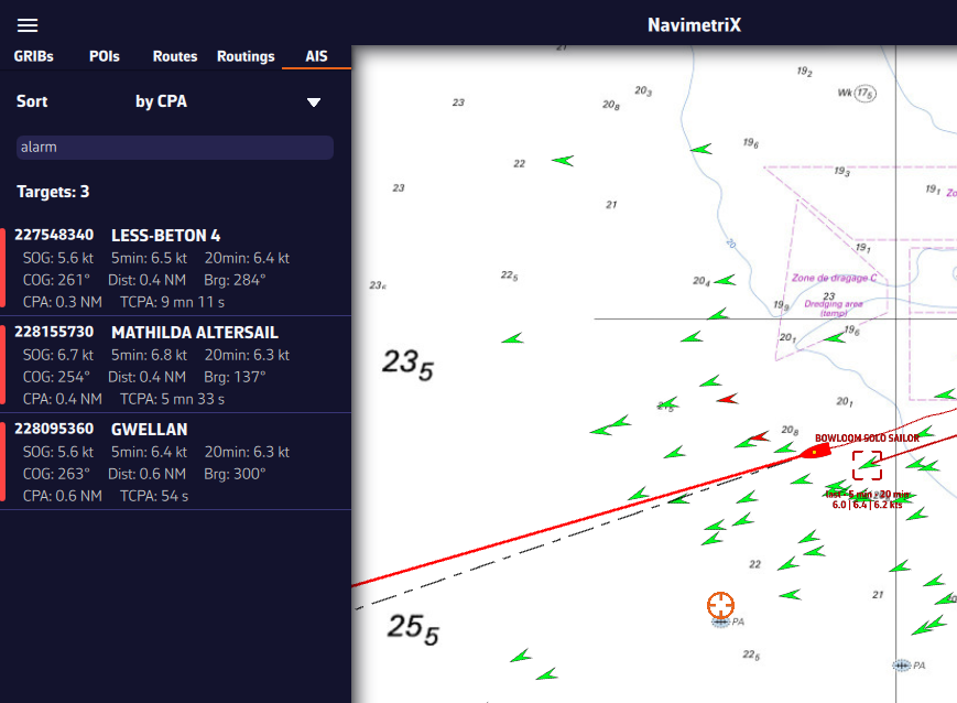
You can display several types of icons on the chart: AIS targets, navigation aids (NavAids), SART (Search And Rescue) distress beacons, AIS targets via the Internet, and “in-situ” weather data stations.
AIS Targets, NavAids, SART
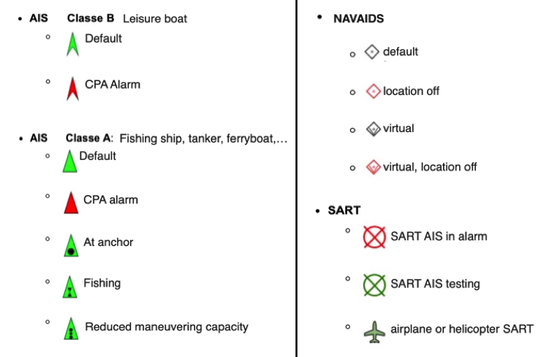
AIS Target over Internet
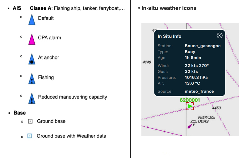
Weather station 'in-situ'
To know more, read our FAQ: How to display "in-situ" weather stations
PermalinkNMEA activation is synchronized on all devices connected to the same Wi-Fi router (NMEA gateway, multiplexer, onboard router). Therefore, disabling NMEA on one device, such as your smartphone, disables NMEA on other devices in use, such as tablets or computers.
You have two options in the above case:
- Disconnect your smartphone from the Wi-Fi router to continue using Navimetrix in Internal GPS mode. You will no longer receive the data stream and your position will be that of your smartphone.
- If your NMEA router is simultaneously connected to the internet via a Cellular SIM card, you should not disable NMEA on your smartphone because synchronization also occurs via the internet.
- Offshore, offline, you can disable NMEA unless your router is connected to a Starlink antenna.
- Close NavimetriX on your smartphone.
Track management is now organised in two places:
- the Tracks panel in the hamburger menu, to manage your recorded tracks (your trips);
- Settings > My Boat > Track, to adjust the track's appearance.
The Tracks panel (hamburger menu)
Open the hamburger menu (☰ top left) and select the Tracks tab.
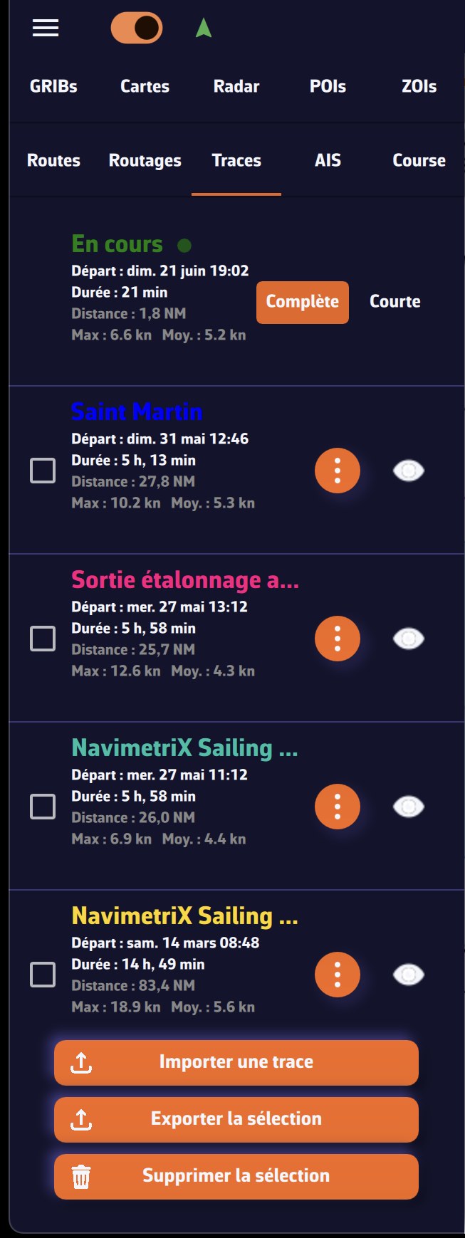
The track currently being recorded appears at the top, marked "Ongoing" with a pulsing red dot. Recording starts as soon as you switch on Navigation mode and stops when you switch it off. For this track you can choose the displayed extent:
- Full: the whole current trip;
- Short: the last 20 minutes (lighter track).
Each saved track shows its name, start date, duration, distance as well as its max and average speed.
For each saved track you have:
- the eye icon: show or hide the track on the map;
- the ⋮ menu (three dots): Details, Rename, Color, Export / Share (GPX) and Delete.
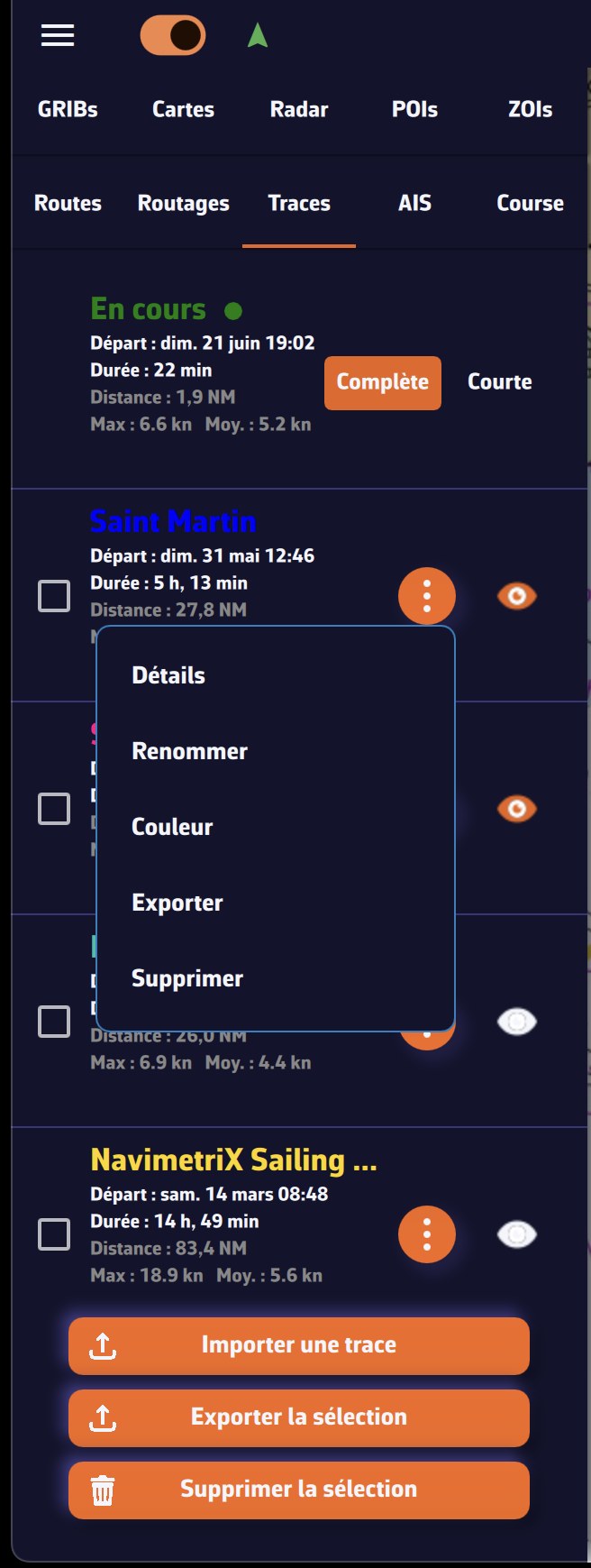
At the bottom of the panel, three buttons act on several tracks at once (tick the boxes on the left to select them):
- Import track: import a GPX file;
- Export / Share selection: bundle the ticked tracks into a single GPX file;
- Delete selection: delete the ticked tracks.
Adjust the track's appearance
Open the Settings (gear button, top right), select My Boat, then the Track section.
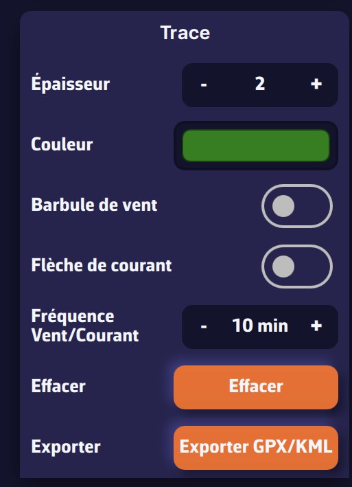
You are able to:
- Adjust the line width (1 to 5)
- Select the track color
- Choose whether or not to display wind barbules on the track
- Choose whether or not to display current arrows on the track
- Adjust the frequency of the wind/current display
- Clear the track
- Export the track (GPX/KML format)
The current track is now always displayed: there is no longer a display switch or a duration setting. For a lighter track, switch the ongoing track to Short (last 20 minutes) in the Tracks panel.
PermalinkConnecting the NMEA multiplexer in Wi-Fi client mode to the Starlink router
Principle
In Wi-Fi "client mode", the multiplexer connects to the Starlink router's Wi-Fi network like any other device. It obtains a local IP address and exposes its NMEA stream via TCP on that network.
NMEA 0183 instruments -> NMEA multiplexer (Wi-Fi client mode) -> Wi-Fi -> Starlink router (192.168.100.1 by default)
- Internet (Starlink WAN)
- Multiplexer → example: 192.168.100.x:10110
- iPad/iPhone with NavimetriX
- Yacht Devices YDNM-02: menu "Network → Wi-Fi → Station mode"
- Actisense W2K-1: menu "Wireless → Client mode"
- Vesper XB-8000: menu "Network → Join existing network"
- Starlink app → Network → Connected devices
- Either via the Starlink router: "static DHCP lease" tied to the multiplexer's MAC address
- Or via the multiplexer itself: assign it a fixed IP within its range
- Host: the multiplexer's IP address (example: 192.168.100.42)
- Port: multiplexer port (example: 10110 - standard NMEA 0183, check according to your device)
- The Starlink router uses "double NAT". This is not an issue for local use — everything stays on the LAN.
- "AP isolation" enabled on Starlink: this must be disabled, as it prevents Wi-Fi devices from communicating with each other.
- The multiplexer's IP changes: use a static DHCP lease by MAC address (in the Starlink app).
- Test the TCP connection to the multiplexer (example: 192.168.100.42:10110)
Step-by-step configuration
1. Switch the multiplexer to Wi-Fi client mode
Depending on the model, via its web interface (often 192.168.1.1 or 192.168.4.1, set to Access Point mode by default):
Enter the SSID and password of the Starlink network.
2. Find the IP address assigned to the multiplexer
After connecting, locate the IP in the Starlink router admin interface:
3. Assign a static IP to the multiplexer (recommended)
To prevent the IP from changing on every restart:
4. Configure NavimetriX
In NavimetriX, set up the NMEA connection via TCP:
Precautions
Checking that everything works
You should see NMEA sentences scrolling by ($GPGGA, $GPRMC, !AIVDM…)
The NMEA stream and internet coexist perfectly — they share the same Wi-Fi network, but traffic is naturally separated (local versus WAN).
PermalinkLaylines are automatically displayed when you have activated a POI using the ‘Go to’ function and you need to tack or jibe to reach your target, upwind or downwind.
Definition
The layline is an ideal course on the water for reaching targets: marks or waypoints. It is an imaginary line that varies depending on the wind, current, and the sailboat's ability to sail upwind or downwind, as determined by its speed polar curve. The layline starts from the target, upwind or downwind, to indicate the course to follow and the point at which a boat must tack or jibe in order to reach the target as quickly as possible.
How it works
By convention, the green layline is the starboard tack, and the red layline is the port tack.
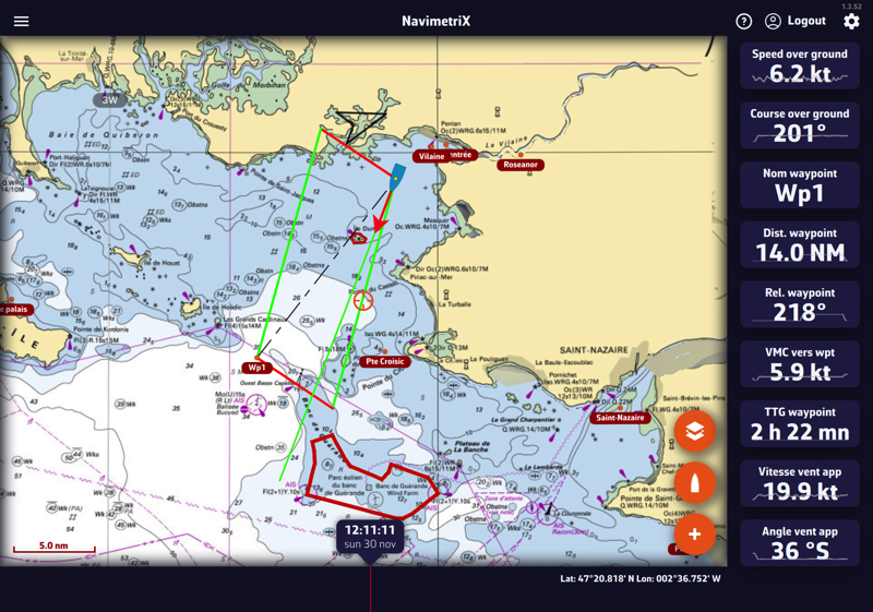
Following this guideline, the distance to be covered by following the best VMG (VMG Max), upwind or downwind, is the same; it is the optimal distance to be covered. If you move outside the laylines, the distance to be covered increases; if you sail within the layline, performance decreases. The angle and heading values vary dynamically with changes in the apparent wind speed and direction.
You can activate the instruments corresponding to the layline data:
- Layline distance: length of the layline before tacking
- Layline time: duration of the layline before tacking
Display
Layline display can be enabled/disabled in the "Layers" menu:
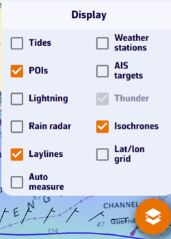
You can send NMEA data to instruments to:
- Control an autopilot by activating navigation to a waypoint.
- Send data from your mobile device's internal sensors (1) to external repeaters.
- Send data to NKE Multigraphic instruments.
In the Settings menu, select the GPS & NMEA option.
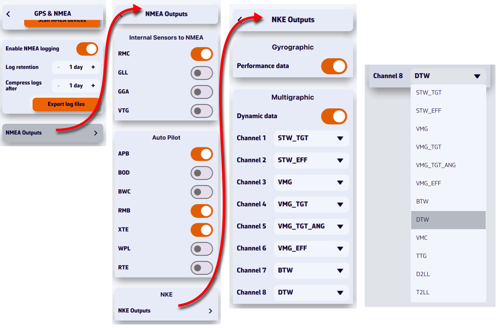
In order to be received by your instruments, the sentences must be transmitted via a bidirectional gateway or multiplexer, usually via Wi-Fi, but also via USB. To be processed, you must first check the sentences allowed by your instruments in their user manual (autopilot, chartplotter, repeater, etc.).
For NKE instruments, you can feed each of the 8 dynamic channels of the NKE Multigraphic from a list of sentences by scrolling down the menu for each channel.
(1) Depending on the mobile device used, mainly smartphones and tablets, the sensors may include:
- Built-in GPS.
- Digital compass.
- 3-axis gyroscope.
- Electronic barometer.
Manual measurement
Using the action button, you can perform several measurements on the chart. Select ‘Add a new measure’ then move the endpoints. The vector displays the distance and true bearing.
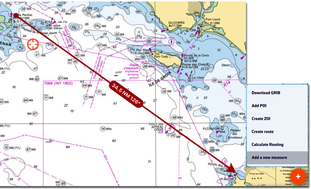
To delete the measurement, tap/click on the data lable of the arrow.
The origin and/or end of the arrow may be magnetized on a POI. In this case, clear the measurement by tapping/clicking on the free end, and if both ends are magnetized on two POIs, simply drag one of the two ends to release and clear it.
Automatic measurement
From the Layers button, check the ‘Auto measure’ display option:
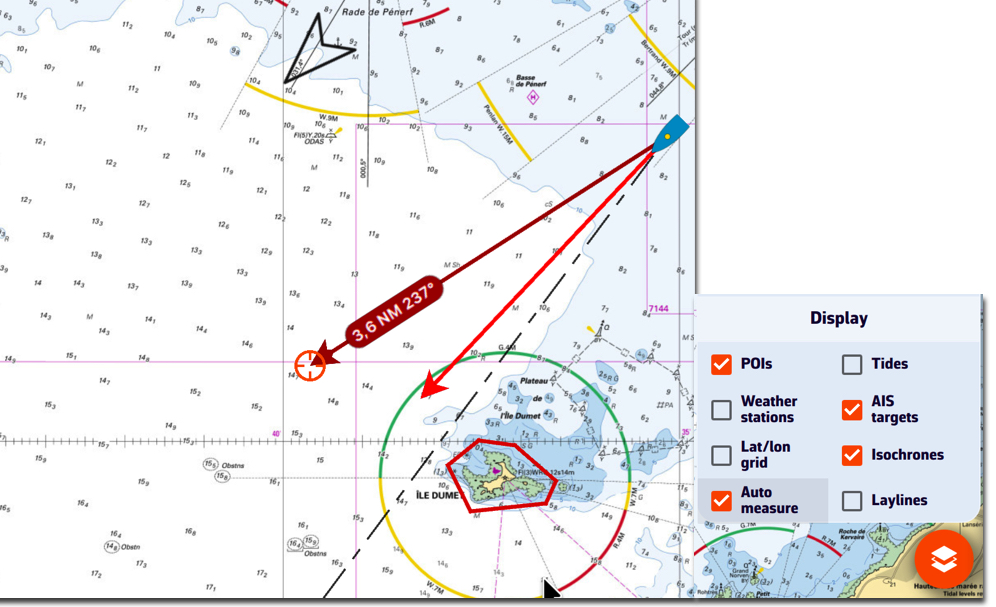
The measurement arrow is automatically displayed from your location toward the target in the centre of the screen. Simply move the chart under the target to the desired location. The distance vector is then displayed for a short time, giving you time to read the distance and true bearing. Each time the chart is moved under the target, the vector is reset.
You can disable the distance vector display by unchecking the ‘Auto measure’ box.
PermalinkDEMO mode allows you to view a navigation routine with moving AIS targets. This gives you an idea of how the application works when you are "at home".
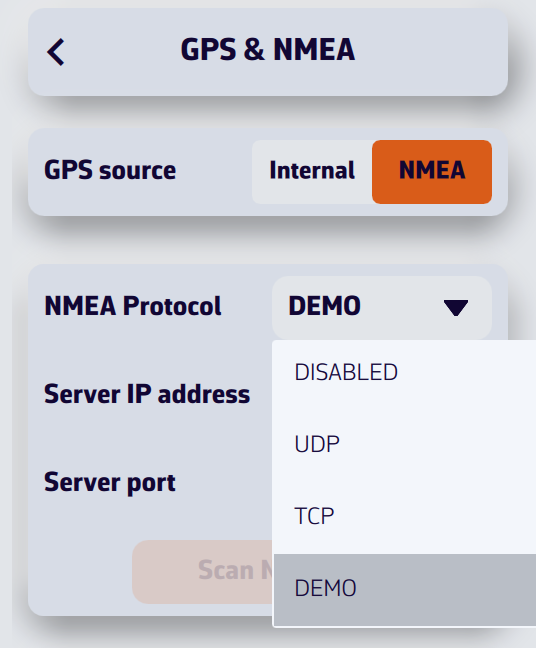
Open the settings and select the GPS & NMEA option. Select GPS source = NMEA.
In the ‘NMEA Protocol’ drop-down menu, select DEMO.
The window will then display a simulated routine allowing you to see NavimetriX in action while navigating, select AIS targets to display CPA prediction points, read target information in the side column list, view navigation data in the instruments, etc.
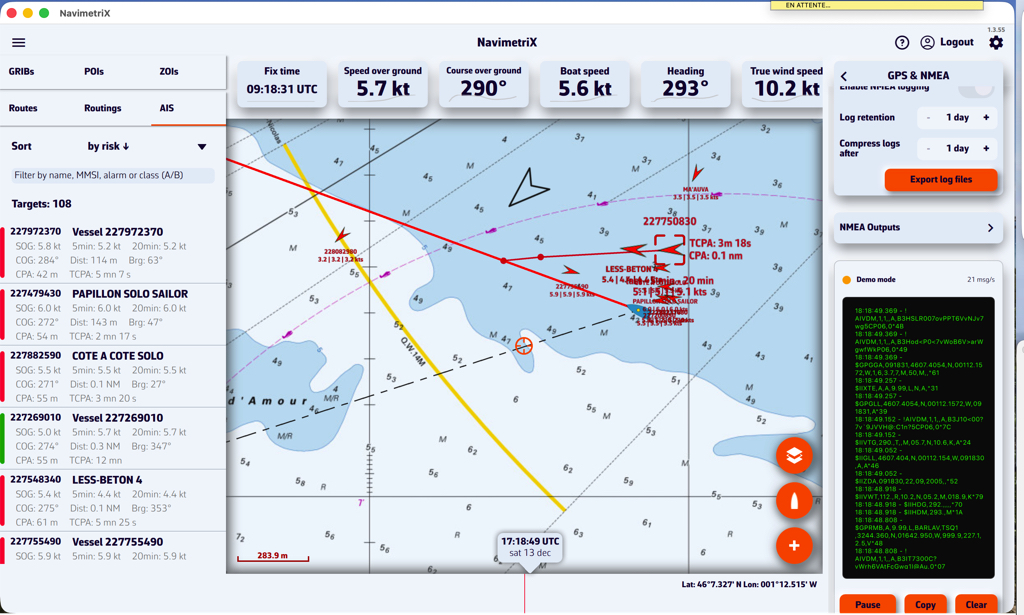
NavimetriX receives navigation data from your instruments via NMEA 0183 sentences. When multiple sentences can provide the same parameter, the app uses the highest-priority source available (1 = first choice). If that sentence isn't received, it falls back to the next priority.
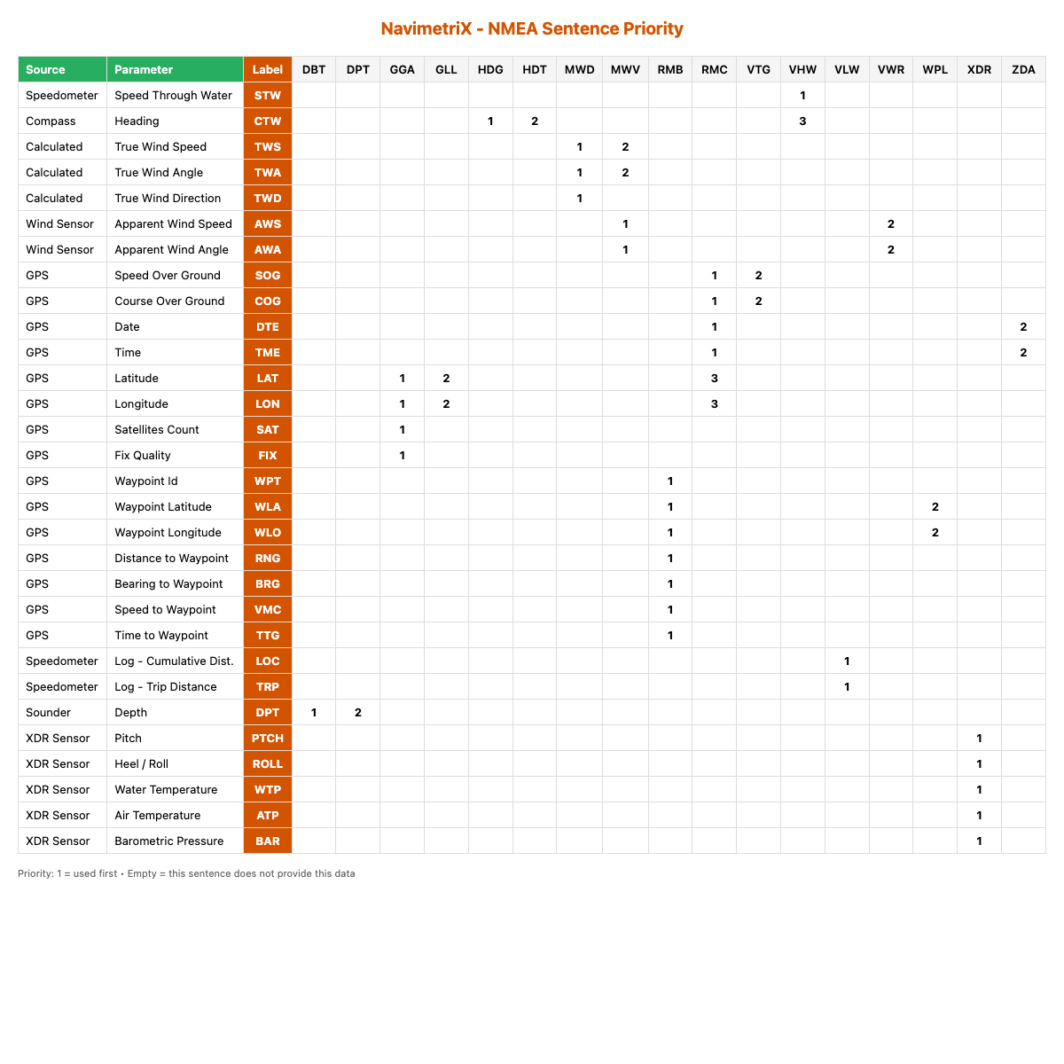
FAQ - NMEA0183 XDR Sentence (Transducers)
What is the XDR sentence?
The XDR (Transducer Measurement) sentence is a generic NMEA0183 sentence used to transmit measurements from various types of sensors (transducers). It allows multiple measurements to be grouped into a single sentence.
What is the general format of the XDR sentence?
$xxXDR,a,x.x,u,n,a,x.x,u,n,...*hhWhere for each transducer group:
- a: Transducer type (one letter)
- x.x: Measured value
- u: Unit of measurement (one letter)
- n: Transducer name (character string)
The checksum (*hh) is mandatory.
Which transducers are supported by NavimetriX?
1. Heel/Pitch
| Field | Value |
|---|---|
| Type | A (Angular) |
| Unit | D (Degrees) |
| Name | PTCH |
Example:
$IIXDR,A,5.2,D,PTCH*XXThis indicates a pitch angle of 5.2°.
2. Roll
| Field | Value |
|---|---|
| Type | A (Angular) |
| Unit | D (Degrees) |
| Name | ROLL |
Example:
$IIXDR,A,-1.1,D,ROLL*XXThis indicates a roll angle of -1.1°.
Combined example (Roll + Pitch):
$IIXDR,A,-1.1,D,ROLL,A,5.0,D,PTCH*743. Water Temperature
| Field | Value |
|---|---|
| Type | C (Temperature) |
| Unit | C (Celsius), F (Fahrenheit), or K (Kelvin) |
| Name | Must contain water (e.g., WATERTEMP, WaterTemp, water) |
Examples:
$IIXDR,C,18.5,C,WATERTEMP*XX
  $IIXDR,C,65.3,F,WaterTemp*XX
  $IIXDR,C,291.65,K,water*XX
4. Air Temperature
| Field | Value |
|---|---|
| Type | C (Temperature) |
| Unit | C (Celsius), F (Fahrenheit), or K (Kelvin) |
| Name | Must contain air (e.g., AIRTEMP, AirTemp, air) |
Examples:
$IIXDR,C,22.0,C,AIRTEMP*XX
  $IIXDR,C,71.6,F,AirTemp*XX
Combined example (Water + Air):
$IIXDR,C,18.1,C,WATERTEMP,C,22.0,C,AIRTEMP*495. Barometric Pressure
| Field | Value |
|---|---|
| Type | P (Pressure) |
| Unit | B (Bars) |
| Name | Must contain baro (e.g., BARO, Barometer, baro) |
Note: The value must be expressed in Bars (1 bar = 1000 hPa). NavimetriX automatically converts it to hPa.
Example:
$IIXDR,P,1.013,B,BARO*XXThis indicates a pressure of 1013 hPa.
How do I combine multiple measurements in a single sentence?
Transducer groups can be chained in the same XDR sentence (up to 10 transducers per sentence):
$IIXDR,A,-2.5,D,ROLL,A,3.1,D,PTCH,C,18.5,C,WATERTEMP,C,21.0,C,AIRTEMP,P,1.015,B,BARO*XXIs the transducer name case-sensitive?
No. Transducer name recognition is not case-sensitive for temperatures and pressure:
WATERTEMP,WaterTemp,watertemp→ all recognizedAIRTEMP,AirTemp,airtemp→ all recognizedBARO,Barometer,baro→ all recognized
Exception: For roll and pitch, the names must be exactly ROLL and PTCH.
Which talker prefix should I use?
NavimetriX accepts all standard talker prefixes (II, GP, HC, etc.). The examples above use $II (Integrated Instrumentation), but $GP, $HC, or others are equally valid.
Summary of accepted formats
| Measurement | Type | Unit | Transducer Name |
|---|---|---|---|
| Pitch | A | D | PTCH |
| Roll | A | D | ROLL |
| Water temperature | C | C, F, or K | contains water |
| Air temperature | C | C, F, or K | contains air |
| Barometric pressure | P | B | contains baro |
You can display a path on the screen showing the maximum cross track error that should not be exceeded.
In the NavimetriX Settings, select the “Alarms” function, set the XTE course deviation to the maximum desired distance on either side of the activated route to a waypoint, then activate the alarm. This instantly displays, depending the zoom level, the XTE zone delimited by red (port) and green (starboard) dotted lines:
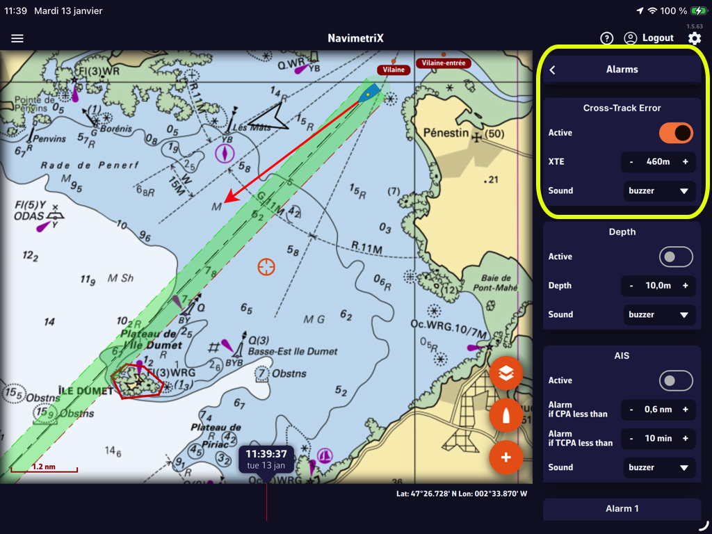
In that example, the value “460m” creates a corridor of 920 meters, or about half a nautical mile. You can select the audible alarm that suits you from the “Sound” drop-down menu.
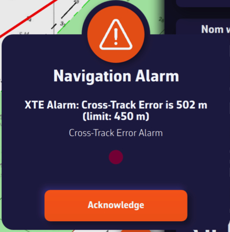
.Leaving the “corridor” triggers an audible and visual alarm that you can disable by tapping/clicking on “Acknowledge” button
PermalinkIf you do not see NMEA sentences scrolling in the NavimetriX NMEA console, this may be related to the limitations of the WiFi module integrated in the box, which is now end of life. This module is no longer fully compatible with certain devices, in particular the most recent mobile devices.
Check the box software version
Before performing any other action, it is essential to verify that your NKE WiFi box is running the latest internal software version. The currently available version is version 2.5. A box running an older version may experience WiFi connection issues.
You can check the version of your box directly on your MultiGraphic or Multi Display, or using the TopLink software. The software update must be performed using the TopLink software.
Download and install the TopLink software
Checking and updating the software of the NKE WiFi box is done using the TopLink software. This software runs only on Windows PCs. To download it, go to the NKE website, click on the hamburger menu at the top right, then access the Technical access section. From there, open the TopLink software page, download the program, and install it on your computer.
Update the NKE WiFi box
Once TopLink is installed and launched, connect to your NKE WiFi box and perform the update to version 2.5.
Case of recent Apple devices
On some Apple devices (iPhone or iPad) running iOS versions higher than iOS 17 (versions released from 2024 onwards), a WiFi security mechanism added by Apple prevents connection to the NKE WiFi box, even when the box is up to date.
In this case, the WiFi must be forced into open mode, without a password.
To do this, press and hold the Init button on the NKE WiFi box for exactly 8 seconds. It is important to respect this duration precisely; you will hear 8 beeps. This action forces the box WiFi into open mode (no password), allowing affected Apple devices to connect.
Finally, restart the box.
Once connected to the box WiFi, access to the NKE WiFi box should be restored and you should see the NMEA sentences in the NavimetriX console.
PermalinkAIS targets over Internet come from the global AISHub network, to which NavimetriX is affiliated.
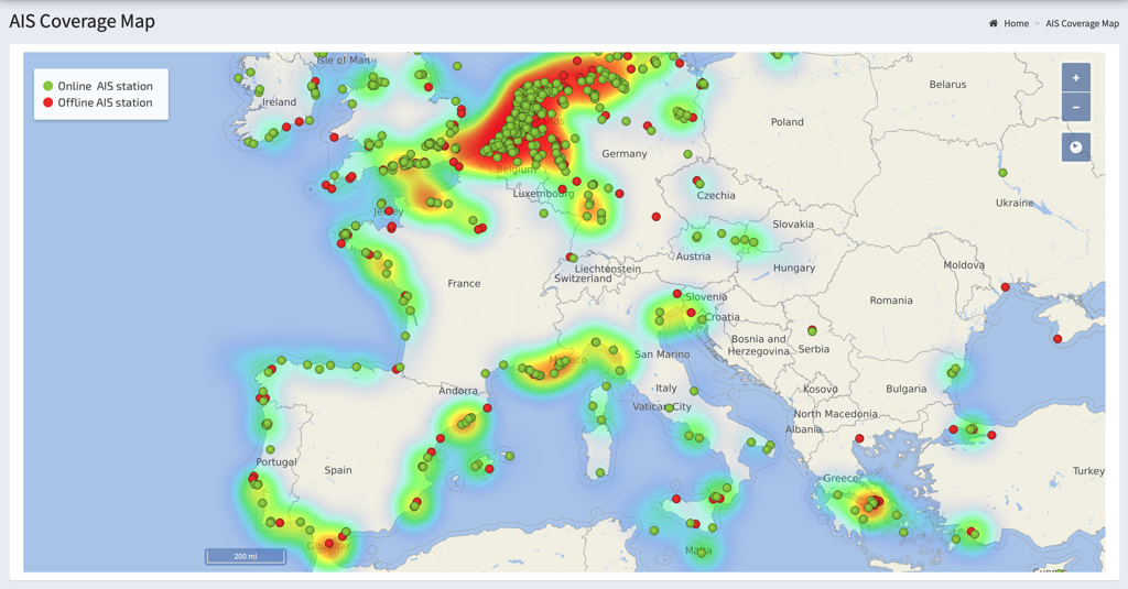
The use and handling of AIS targets over Internet is exactly the same as for AIS targets received on board using an AIS receiver that transmits NMEA data to the application. For more details, see:
How to display AIS targets? in this FAQ.
Open the Settings panel (gear button at the top right)
- Select the AIS option
- Enable AIS over Internet
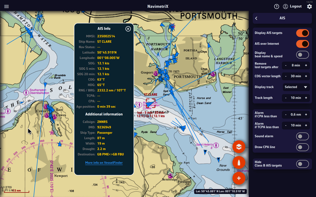
Cautions:
AIS targets over Internet should be considered for informational purposes only. Time delays due to Internet transfer speeds make them unsuitable for navigational safety, whereas reception on board by a dedicated receiver is at VHF frequency in real time.
They are therefore represented by blue icons to differentiate them from green AIS targets icons received directly.
For more details, see: What do the icons displayed on the chart mean in this FAQ?
PermalinkA slider allows you to turn Navigation Mode on and off. The goal is to prevent mobile devices from draining their batteries unnecessarily when certain navigation functions are not in use, such as when running route simulations, analyzing weather data, etc.
Navigation Mode
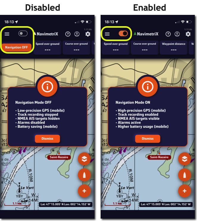
When Navigation mode is turned off, the GPS updates the location only every 30 seconds instead of every second.
Of course, don’t forget to turn Navigation mode back on as soon as you set off.
GPS Accuracy Indicator
An arrow icon indicates the GPS status on mobile devices:
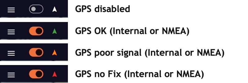
NMEA Data Alarm
An NMEA data reception alarm can be enabled to warn of data loss for a customizable period of time.
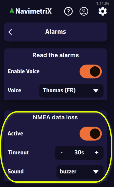
A drop-down menu allows you to select the appropriate sound alarm.
Permalink
As seen in the Cap Martinique race, race instructions typically include details on Traffic Separation Schemes (TSS) that are prohibited along the course. Failure to comply with these zones results in severe penalties, as competitors’ track data serves as irrefutable proof.
It is therefore essential to plot the exact coordinates provided in these race instructions on the electronic charts, and not those entered by hand as one might do in Navimetrix. The app offers a feature to import ZOIs in text format for all TSS specified in the race instructions.
1. Copy the TSS coordinates from the Race Instructions
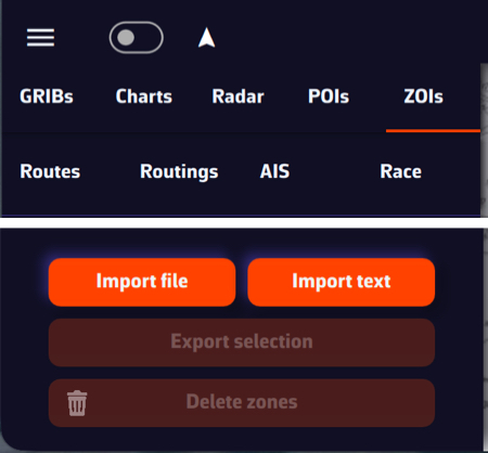
- Select the section of the race instructions containing the TSS description
- Select the text and copy it
- Open the left panel using the ≡ hamburger button
- Select the ZOIs tab
- Tap or click the “Import text” button at the bottom of the window
2. Import text
- Paste the copied content into the window that opens
- If necessary, format the text (there may be unnecessary blank lines)
- You can optionally shorten the name of each TSS in this window so that it appears more compact in the NavimetriX ZOIs window.
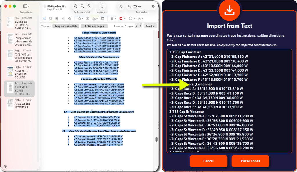
- Tap or click the “Parse Zones” button to check
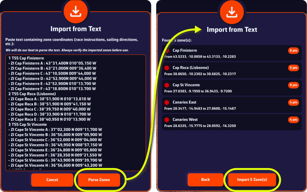
- Tap/click on "Import x Zone(s)" button
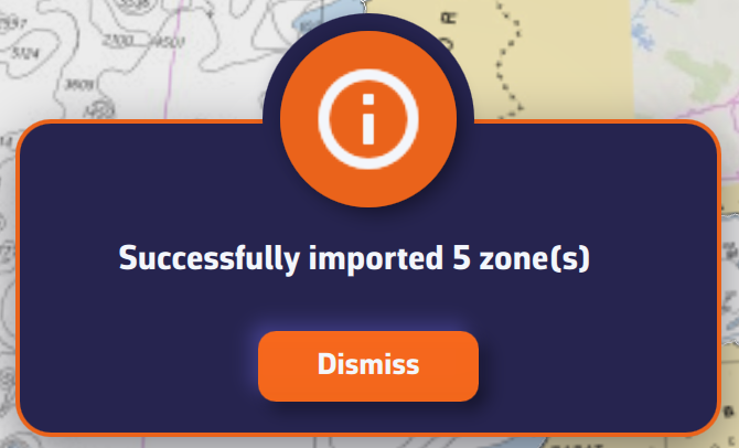
You can now view the TSS in the ZOI list and on your chart.

A tip: if you previously created a TSS zone at the same location as the race instructions, disable its display or delete it to prevent its coordinates from interfering with those of the race instructions, which are the only official source.
PermalinkNavimetriX includes a comprehensive MOB (Man Overboard) function, with drift tracking, search pattern and AIS integration. Here's how to use it.
1. Enable the MOB button
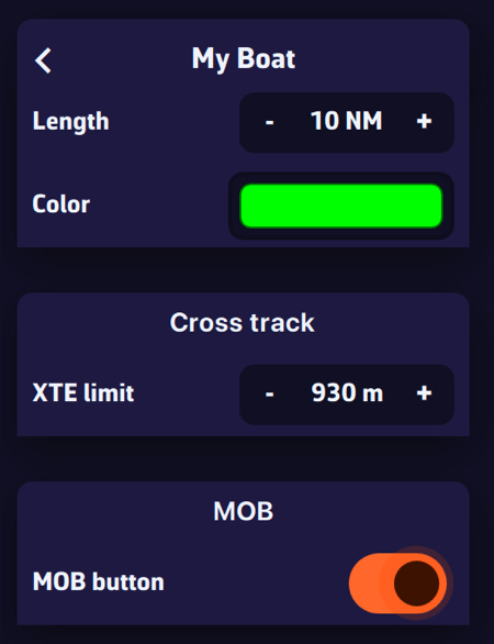
The MOB button is not displayed by default. To enable it:
- Go to Settings → Navigation → My Boat → MOB
- Enable the MOB Button option

The red MOB button then appears at the bottom left of the chart, in Navigation mode only.
2. Trigger MOB
To trigger MOB, press and hold the MOB button for 1.5 seconds. A progress ring fills around the button to indicate progress. This long-press action is intentional to prevent accidental activation.
A short tap simply displays a tooltip reminding you to hold the button.
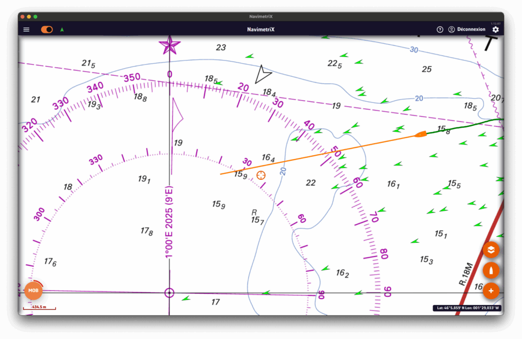
3. What happens when MOB is triggered
As soon as MOB is activated, several actions are performed automatically:
- MOB marker: a point of interest is created at the boat's current GPS position (e.g. "MOB 14:32:58")
- Active waypoint: the MOB position is set as the Goto waypoint, with a route line to the MOB
- Auto zoom: the chart centres and zooms to the MOB position
- Timer: an elapsed time counter starts immediately (displayed in red)
- Drift tracking: drift calculation begins (see next section)
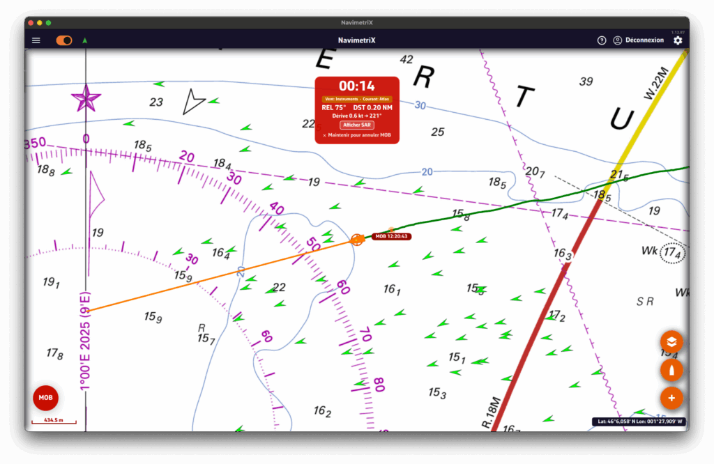
4. The MOB dashboard (HUD)
An information banner appears at the top of the chart with essential data:
- Elapsed time: displayed in large red format (MM:SS)
- Bearing (BRG): heading to steer towards the MOB position
- Distance: distance to the MOB (in nautical miles, or metres when < 0.1 NM)
- Drift data: estimated drift speed and direction
- Mode badge: indicates the data source (GRIB wind, current, AIS...)
- Search button: to show or hide the search pattern
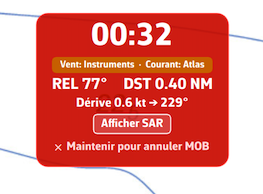
5. Drift tracking
NavimetriX estimates the probable position of the person in the water taking into account:
- Wind: using GRIB data or onboard instruments. Leeway is calculated at 3% of the true wind speed with a 10° divergence, in accordance with international search and rescue standards.
- Current: using GRIB data, tidal atlas or onboard instruments.
On the chart, you will see:
- An orange drift line connecting the initial MOB position to the estimated position
- An orange circle around the estimated position, whose radius increases over time (growing uncertainty)
The estimated position is updated every 30 seconds and the Goto waypoint is automatically adjusted.
6. Search pattern
NavimetriX can display an expanding square search pattern, compliant with international search and rescue procedures (IAMSAR).
To display it, tap the "Search" button in the MOB banner. The pattern is centred on the estimated drift position (or on the initial MOB position if no drift data is available).
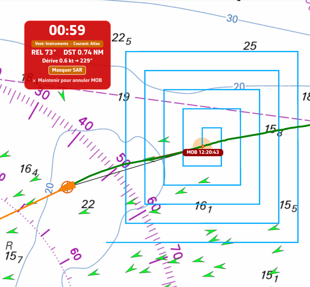
7. MAYDAY reminder
60 seconds after MOB activation, if the situation is not resolved, a yellow banner appears as a reminder to consider a MAYDAY call on VHF channel 16 (RYA recommendation).
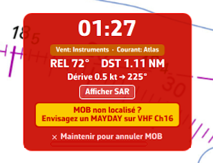
8. AIS MOB integration
If an AIS MOB beacon (personal or SART type) is detected nearby, NavimetriX reacts automatically:
- An audible alarm sounds
- An alert dialogue displays the beacon's position
- MOB mode activates automatically if not already active
- The AIS position is tracked in real time (updated every 5 seconds)
If the AIS signal is lost, NavimetriX automatically switches to drift estimation mode after 60 seconds.
The mode badge in the MOB banner changes colour depending on the situation:
- Green: AIS MOB beacon detected and tracked
- Red: AIS MOB signal lost
- Orange: drift data available (wind/current)
- Grey: no drift data available
9. Cancel MOB
To cancel MOB mode, press and hold the "Hold to cancel MOB" text in the MOB banner for 1.5 seconds. A progress bar confirms the cancellation.
Cancelling deactivates tracking, removes the Goto waypoint and hides the MOB banner.
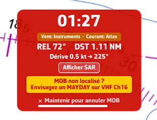
10. Practical tips
- Enable the MOB button before heading out to sea in the settings, so it is immediately accessible in an emergency
- Load a GRIB file for your sailing area: GRIB wind and current data significantly improve drift calculation accuracy
- Equip yourself with an AIS MOB beacon: it provides real-time tracking of the person in the water, far more accurate than drift estimation
- The MOB button only appears in Navigation mode with an active GPS position
What is Race Tracking?
Race Tracking allows you to follow offshore sailing races in real-time directly on the NavimetriX chart. You can import race definitions, download position reports automatically or manually, and view rankings based on distance to finish.
What file formats are supported?
Race Tracking supports the Adrena format, which is the standard used by most offshore race organizers:
- .dcc files - Race definition with competitor list, classes, IRC ratings, and download configuration
- POSADRENA files - Position reports with boat coordinates and timestamps
What is a .dcc file?
A .dcc file (Adrena competitor description) contains all the race information:
- Race name and date
- List of competitors with their boat name, class, skipper, and IRC rating (TCC)
- Display colors for each boat
- FTP or HTTP server configuration for automatic position downloads
Example entry for KORNOG2, a Pogo 12.50 racing in IRC Two class:
KORNOG2;IRC Two;1;3;1;;;8;;1.170;O;Gilles Colubi & Yvan Osselin;;;Race organizers typically provide .dcc files on their website or via email before the race start.
What is the POSADRENA position format?
POSADRENA is the standard format for position reports. Each file contains the latest positions for all competitors:
POSADRENA
  1;8;25.1873N;19.0716W;01/13/26 14:00:01
The fields are: race ID; boat ID; latitude; longitude; timestamp.
Important: Coordinates use the Adrena format (degrees.minutes), not decimal degrees. For example, 25.1873N means 25° 18.73' N (not 25.1873°).
How do I import a race?
To import a race:
- Go to Settings → Race Tracking
- Tap Import Race (.dcc)
- Select the .dcc file from your device
- The race and all competitors will be imported
How do I download position reports?
There are three ways to get position updates:
1. Automatic download (FTP/HTTP)
If the .dcc file contains server configuration, enable Auto-download and set the polling interval. NavimetriX will automatically fetch new positions.
2. Direct URL download
Some tracking systems (like YB Tracking) provide a direct URL that always contains the latest positions. Enter this URL in the connection settings and tap Download Now. NavimetriX will fetch the file and filter out positions already in the database.
Example URL format: https://yb.tl/racename-adrena.txt
3. Manual import
Tap Import Positions and select one or more POSADRENA files from your device. You can select multiple files at once to import a full position history.
How do I view competitors on the chart?
Once positions are imported:
- Open the Race List from the Race Tracking menu
- Toggle visibility for individual boats or use Show All / Hide All
- Competitors appear on the chart with their track history
- Tap a boat icon to see details (position, speed, course)
How are rankings calculated?
Rankings are based on Distance To Finish (DTF):
- Select a route that represents the race course
- DTF is calculated as the distance from each boat's current position to the finish, following the remaining waypoints
- Boats are ranked by ascending DTF (lowest distance = leading)
To enable rankings:
- Create a route matching the race course (or import the official route)
- In Race Settings, select the route name
- Enter the race start date and time (UTC)
- Rankings become available in the Race List
How does IRC corrected time work?
IRC (International Rating Certificate) uses a Time Correction Coefficient (TCC) to handicap boats of different performance levels. This allows boats of different sizes and types to compete fairly.
The formula is: Corrected Time = Elapsed Time × TCC
For example, KORNOG2 has a TCC of 1.170. If the boat finishes in 10 days (240 hours):
- Elapsed time: 240 hours
- Corrected time: 240 × 1.170 = 280.8 hours
A TCC greater than 1 means the boat is "fast" and gets penalized. A TCC less than 1 means the boat is "slow" and gets a time bonus.
For boats still racing, NavimetriX estimates the corrected time based on current VMC (Velocity Made good on Course) to project the finish time.
Why don't I see any boats on the chart?
Check the following:
- Make sure you have imported position reports (not just the .dcc file)
- Check that boat visibility is enabled in the Race List
- Zoom and pan the chart to the race area (boats may be far from your current view)
- Verify the positions were imported successfully (check the position count in Race List)
Why are speeds showing as unrealistic values?
Speed is calculated from position history. Unrealistic values usually indicate:
- Wrong start date/time: Check that the race start datetime in settings matches the actual race start (UTC timezone)
- Insufficient positions: At least 2 positions are needed to calculate speed
- Position errors: Occasionally, tracking systems report erroneous positions
Can I edit competitor information?
Yes, tap on a competitor in the Race List to edit:
- Boat name, class, and skipper
- IRC rating (TCC)
- Display color
- Arrival status and time
- Retirement status
Changes are saved to the database. You can also export a modified .dcc file to share with others.
PermalinkNMEA data streamed by an NMEA gateway, a multiplexer, or any other instrument broadcasting on a serial port via a USB connection is supported.
Prerequisites
Normally, direct transmission of the data stream to a serial port does not require a driver.
Setup
Open Settings by tapping the gear icon, then select GPS & NMEA. Once connected and data transmission enabled, select:
- GPS Source = NMEA
- NMEA Protocol = SERIAL
Press the “Scan NMEA Devices” button.
- Serial Port = the detected port should appear in the window.
- Baud Rate = 4800 bps by default.
The data stream should scroll in the lower window.
PermalinkThe anchor drag alarm monitors your boat's position at anchor and alerts you if it drags.
NavimetriX draws a swing zone around the anchor, triggers a siren if the boat leaves the zone, can send an SMS alert, and lets you track the boat remotely from another device.
The anchor drag alarm is reserved for the Premium subscription.
Dropping the anchor
You must be in Navigation mode, with a GPS fix and the boat almost stationary (speed below 2 knots).

- Once the boat is anchored, tap the + button (bottom right of the chart) then Drop anchor.
- The anchor is placed ahead of the bow (on the heading axis) and a "Anchor DD/MM hh:mm" POI is created.
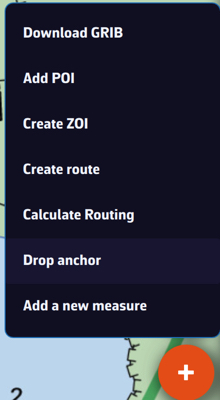
The swing zone
Once the anchor is dropped, a banner appears at the top of the screen and a swing zone is drawn around the anchor. You can choose the shape of the zone:
- Circle — a single radius around the anchor (default radius: 40 m).
- Hexagon — for a custom-shaped zone.
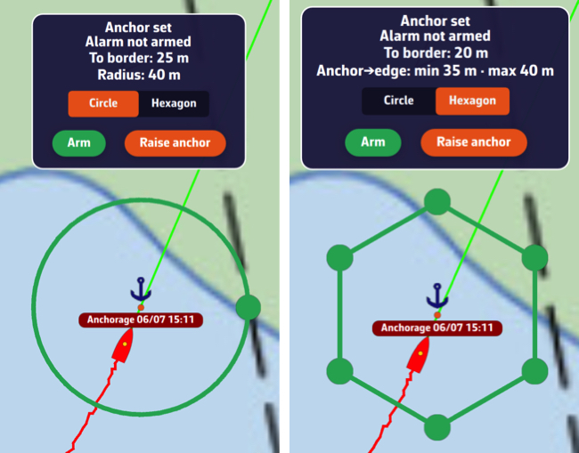
The banner constantly displays the zone's radius and the distance to the edge. Adjust the radius to the length of chain paid out, taking into account the high tide height in tidal areas, plus a safety margin. As a reminder:
- at least 3 x the water depth for all-chain rodes
- at least 5 x the water depth for mixed rope + chain rodes
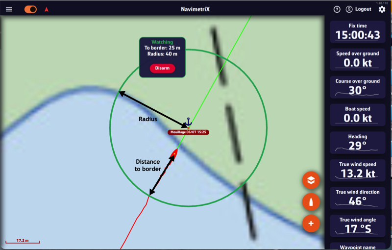
Arming and monitoring
As long as the alarm is not armed, the banner shows "Anchor dropped · Alarm not armed". To activate it, press and hold the Arm button on the banner. The status changes to "Monitoring".
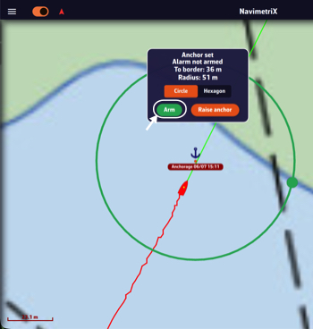
Important: the armed/disarmed state is local to the device. Arming the alarm on your phone does not arm it on the other devices on your account: each device decides on its own whether it monitors and sounds the alarm.
Dragging
If the boat starts dragging, as soon as it leaves the zone the alarm triggers after an adjustable confirmation delay: audible siren, SMS sent (if configured), the banner switches to “DRAGGING” and NavimetriX shows the distance from the anchor relative to the limit.
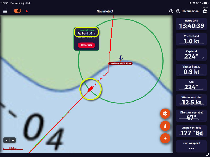
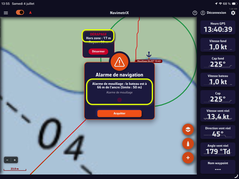
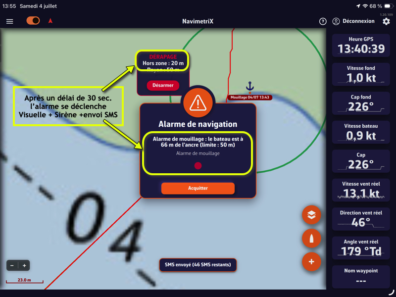
Anchor settings
The settings are found under Settings ▸ Alarms, Anchor section:
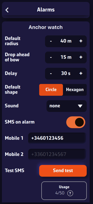
- Default radius — the radius of the swing circle when the anchor is dropped (default 40 m).
- Ahead of the bow — the distance at which the anchor is placed ahead of the boat, on the heading axis (default 15 m).
- Delay — how long the boat must remain outside the zone before the alarm sounds (default 30 s), to avoid false alerts.
- Default shape — Circle or Hexagon.
- Sound — the alarm ringtone to select.
SMS alert
In addition to the local siren, NavimetriX can send an alert SMS to relatives or to another phone on board. Under Settings ▸ Alarms, Anchor section:
- Enable SMS on alarm.
- Enter one or two numbers in Mobile 1 and Mobile 2, in international format (e.g.
+33612345678). - Check with Test SMS ▸ Test: a test message is sent immediately.
If the boat drags, the SMS contains the boat's position, bearing and distance from the anchor, plus a Google Maps link to the boat. Up to 3 SMS are sent per incident: immediately, then at +30 min and +60 min as long as the alarm remains active.
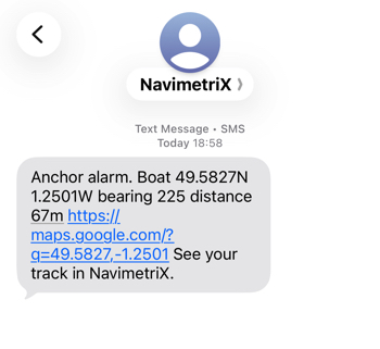
A quota of 50 SMS per rolling 12 months is included. The Usage X/50 counter shows your consumption; once the quota is reached, the app displays "Annual SMS limit reached" (the local siren keeps working regardless).
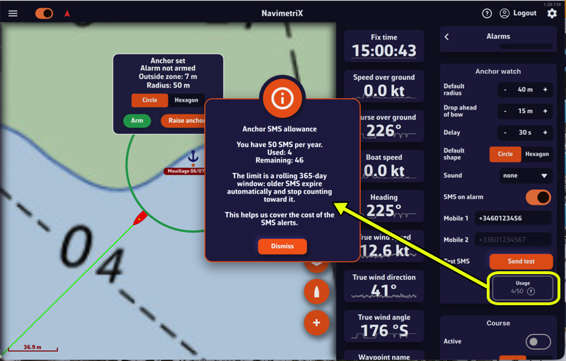
Tracking the boat remotely: "At anchor"
When the boat is at anchor and in Navigation mode, the onboard device shares its position with the other devices connected to the same NavimetriX account. On those devices, an "At anchor" track automatically appears at the top of the Tracks tab.
It shows, read-only:
- the boat's track over the last few hours (swing movements, any dragging);
- the swing zone (circle or hexagon) and the anchor;
- the boat's last known position, oriented to its heading.
Handy for keeping an eye on the boat while relaxing at a restaurant or with friends. A simple tap on the boat icon shows the instantaneous date, speed and heading, tapping the boat button recenters the chart on the anchored boat, and a long press frames the whole swing zone. The "At anchor" track disappears as soon as you raise the anchor or exit Navigation mode on board.
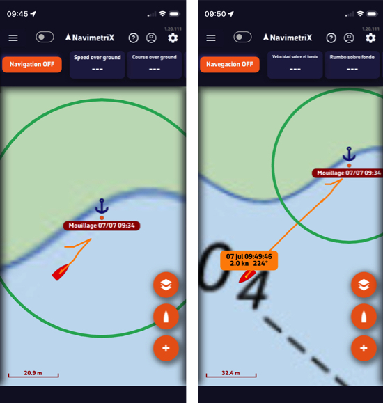
Raising the anchor
When leaving the anchorage, press and hold the Raise anchor button on the banner. The anchoring is closed, the swing zone disappears, and the "At anchor" track is cleared on the other devices.
How to move the anchor?
As long as the alarm is not armed, you can move the anchor using the "Move POI" menu. The swing zone follows the move, so the anchor always stays at the center of the circle.
- Tap the anchor POI.
- Tap "Move POI".
- Drag the POI on the screen. Once released, the swing zone repositions around the new anchor position.