Ensemble routing may seem impressive: 31 route calculations in a single operation! In practice, it is as easy as a conventional routing. Here is how to do it, step by step.

Step 1: Download the GEFS model

• Open the GRIB file download menu.
• Select:
  • Type: Ensemble
  • Coverage: Global
  • GEFS 0.50° model (ensemble)
• Choose the desired time period
• Press: Download GRIB

The average GRIB file downloads like any other model; you don’t need to do anything special.

Step 2: Configure and launch routing

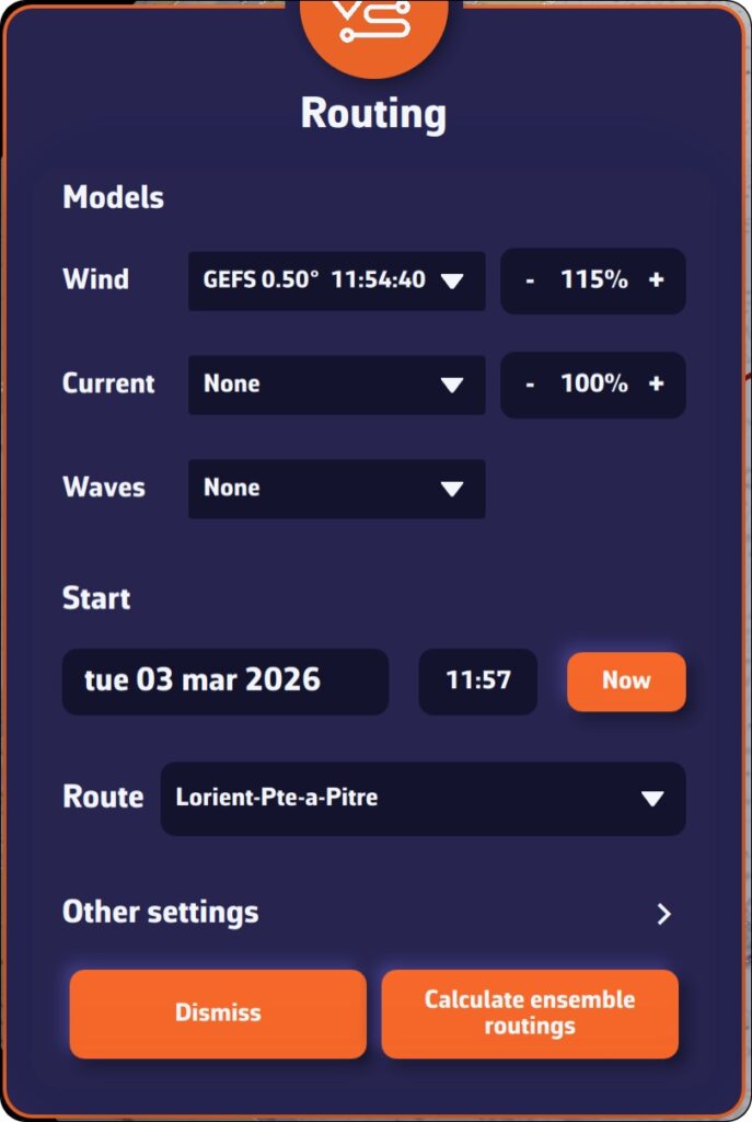
Open the routing window and configure your routing as usual: starting point, destination, ship’s polar curve, start date and time, etc.

NavimetriX automatically detects that you are using a GEFS model. The calculation button changes to display “Calculate ensemble routing.”

Start routing: NavimetriX handles everything!

1. Download the control run (gec00) and calculate its optimal route.
2. Download and calculate the 30 perturbed members, one by one.
3. Combine the results and display them on the chart.

The whole process is fully automated. Downloading each member takes only a few seconds, and route calculation is very fast. You can follow the progress in real time and see the routes appear one by one on the chart.

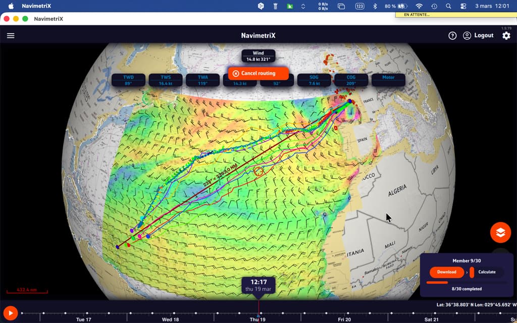
Step 3: Track progress

A compact progress panel appears at the bottom right of the screen. It displays the following in real time:

• Current phase: downloading or calculating
• Current member in progress: “Member 12/30”
• A progress bar for downloads

You can cancel the operation at any time if necessary.

How to interpret the results on the chart

Once the calculation is complete, the chart displays two key elements:

“Spaghetti” routes

Each member is represented by a distinct colored line (the colors are distributed across the entire spectrum to differentiate them clearly). Together, they form a bundle of routes — hence the nickname “spaghetti.” At a glance, you can see:

• Closely spaced routes = high confidence. Regardless of the weather scenario, the optimal route passes through the same location.
• Widely spaced routes = high uncertainty. The optimal route depends heavily on actual weather developments.
• Two distinct groups = two possible weather scenarios, with fundamentally different route strategies.

When the “spaghetti” routes converge, outside of waypoints, confidence is high.

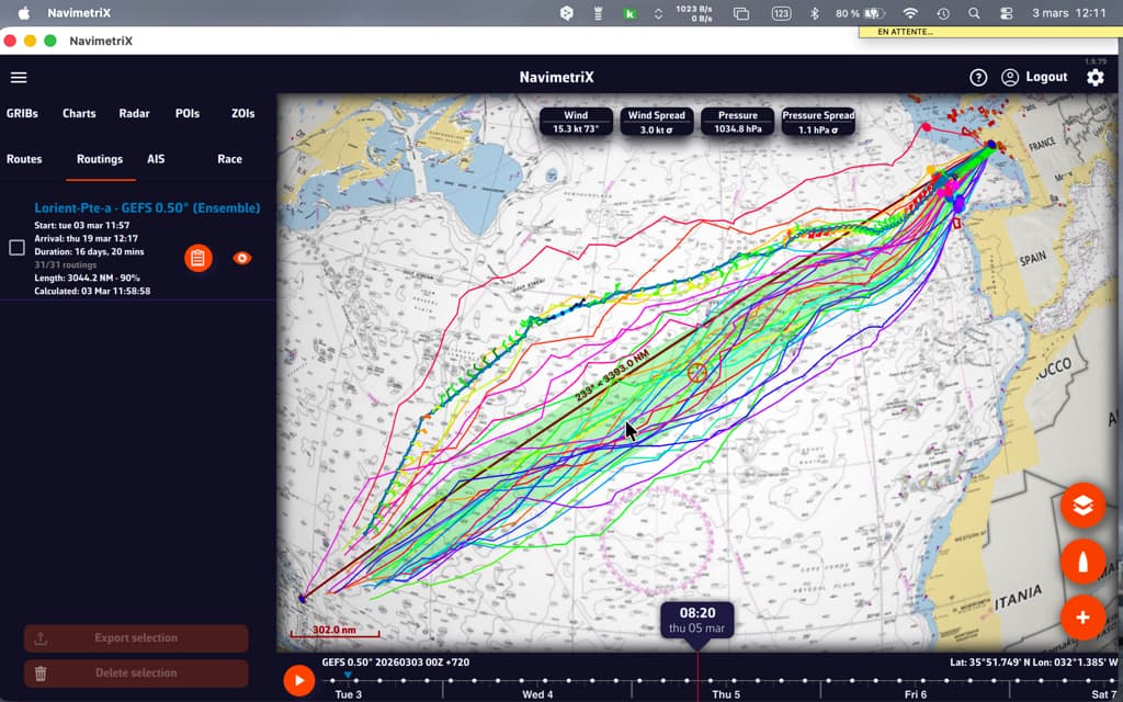
The confidence corridor

Overlaid on top, a semi-transparent green corridor represents the range of ±1 standard deviation. Statistically, approximately 68% of routes fall within this corridor. The 20% of members furthest from the mean are automatically excluded from the calculation to prevent extreme scenarios from distorting the visualization.

The corridor gives you an immediate reading:

• Narrow corridor = reliable route, little variability between scenarios.
• Wide corridor = high uncertainty, the optimal passage zone is vast.
• Corridor gradually widening = confidence decreases over time (typical beyond 4-5 days).

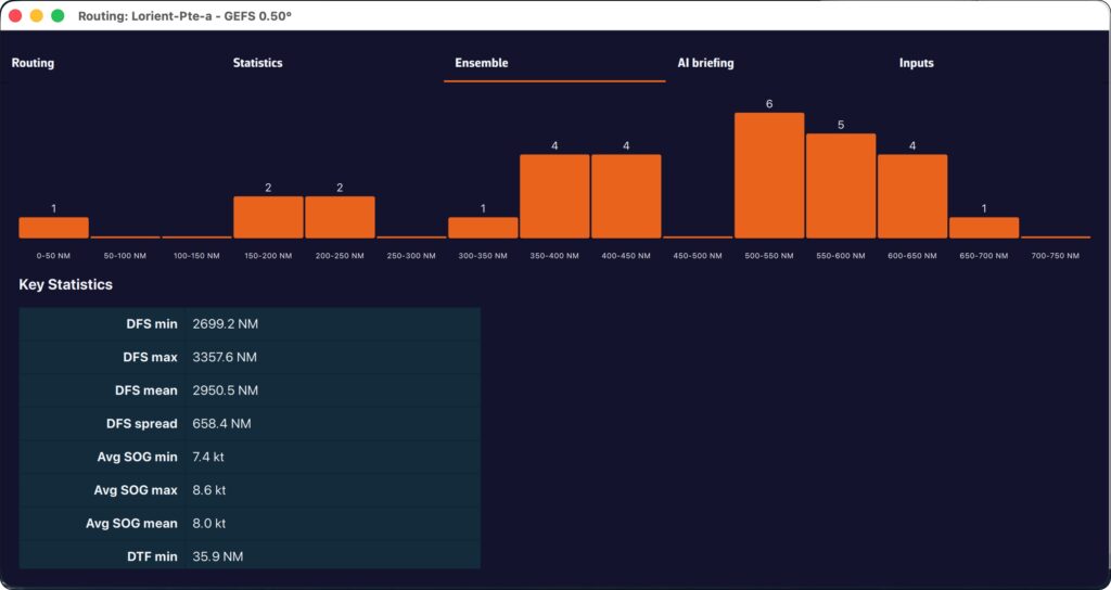
Interpreting statistics

The “Ensemble” tab of the routing table provides a detailed analysis of the 31 scenarios:

• Members who reached the destination: what percentage of the 31 scenarios allowed the destination to be reached? If only 60% reached it, this is a warning sign.
• Distribution of durations: minimum, maximum, average, and median duration. A large min-max spread means that timing is very uncertain.
• Times Arrival (ETA): the earliest and latest, to plan your arrival at the port.
• Control run vs. ensemble average: if the control is significantly faster than the average, the “ideal” forecast is probably optimistic.
• Histogram: visualization of the distribution of durations (or remaining distances if few members reach the finish).

Helpful tips

When should you use ensemble routing?

• Crossings lasting more than 72 hours: uncertainty increases over time, so ensemble routing makes perfect sense.
• Unstable weather conditions: passing fronts, developing low-pressure systems, changing wind patterns.
• Go/no-go decision-making: before a departure, ensemble routing helps you objectively assess the level of risk.
• Medium- and long-term planning: for a crossing lasting more than 5-7 days, observe the daily evolution of member convergence.

Best practices for reading:

• Don’t look for “the best route” among the 31 — look for the area of consensus.
• Use the time slider to see how the routes diverge over time: the first few days are often close, then the gap widens.
• Rerun the ensemble routing when new GEFS data becomes available (every 6 hours) to see if confidence increases or decreases.
• Combine with the spread of wind and pressure displayed on the chart to identify areas of high uncertainty.

Ensemble routing in NavimetriX transforms an analysis that was traditionally reserved for experts into a visual and intuitive tool. With a single click, you can switch from a single forecast to a comprehensive view of all possible options, allowing you to navigate with confidence, even when the weather is not.

———

See also: What is an ensemble weather model…