How to Perform Effective Routing

Basic Principle

Routing is a navigation aid that can serve two different — but not necessarily contradictory — purposes:

• On passage: comfort and safety, avoiding sea and wind conditions that the boat and crew cannot handle,
• Racing: performance, the best efficiency for the best passage time.

Routing is like a cooking recipe: you first need good ingredients:

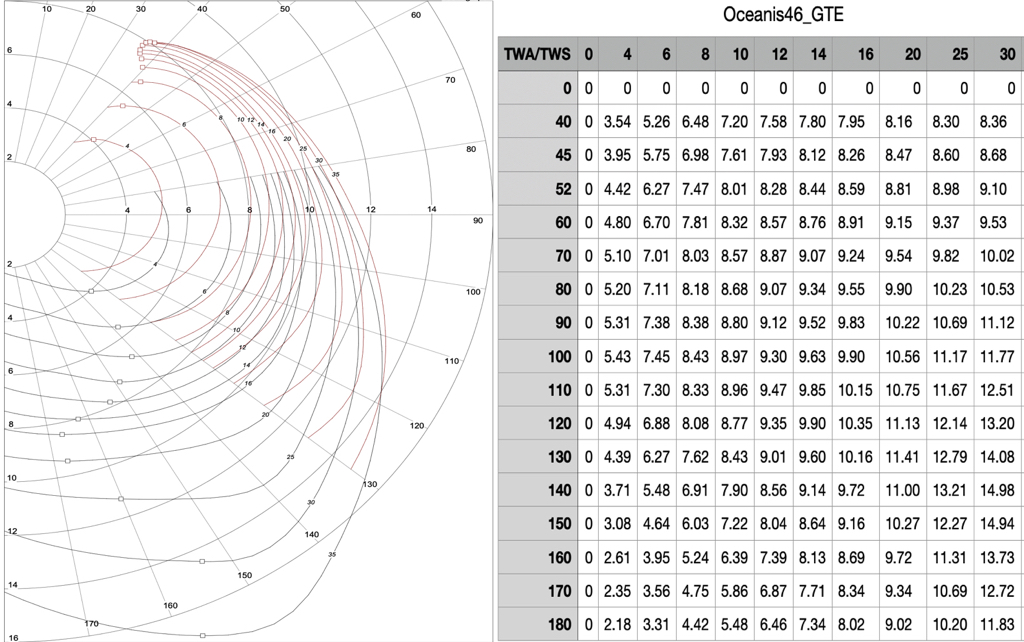
• A speed polar containing the theoretical target speeds the boat can achieve based on true wind speed (TWS) and the sailing angle relative to that wind direction (TWA).
• A route with a minimum of waypoints: preferably only departure and destination. Intermediate waypoints should only be used for mandatory passage points.
• Several GRIB files broadly covering the route: wind, waves, currents — the most recent available, with a time horizon sufficient for the approximate duration of the passage.
• A departure date within the temporal coverage of the GRIB files and as early as possible.

The Recipe

The recipe is based on a routing algorithm — a clever calculation whose inner workings are classified top secret. This calculation determines an optimised route by combining wind values and directions, currents and waves with the boat’s speed polar values, along a course from departure to destination.

It also integrates a number of settings that allow the navigator to add constraints to the data used by the calculation and to fine-tune certain parameters.

Implementation

Polar

Route

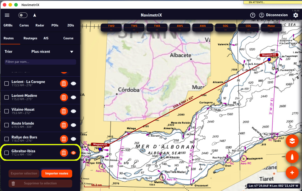
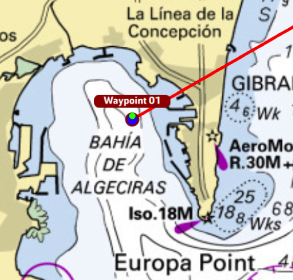
Departure point

Arrival point

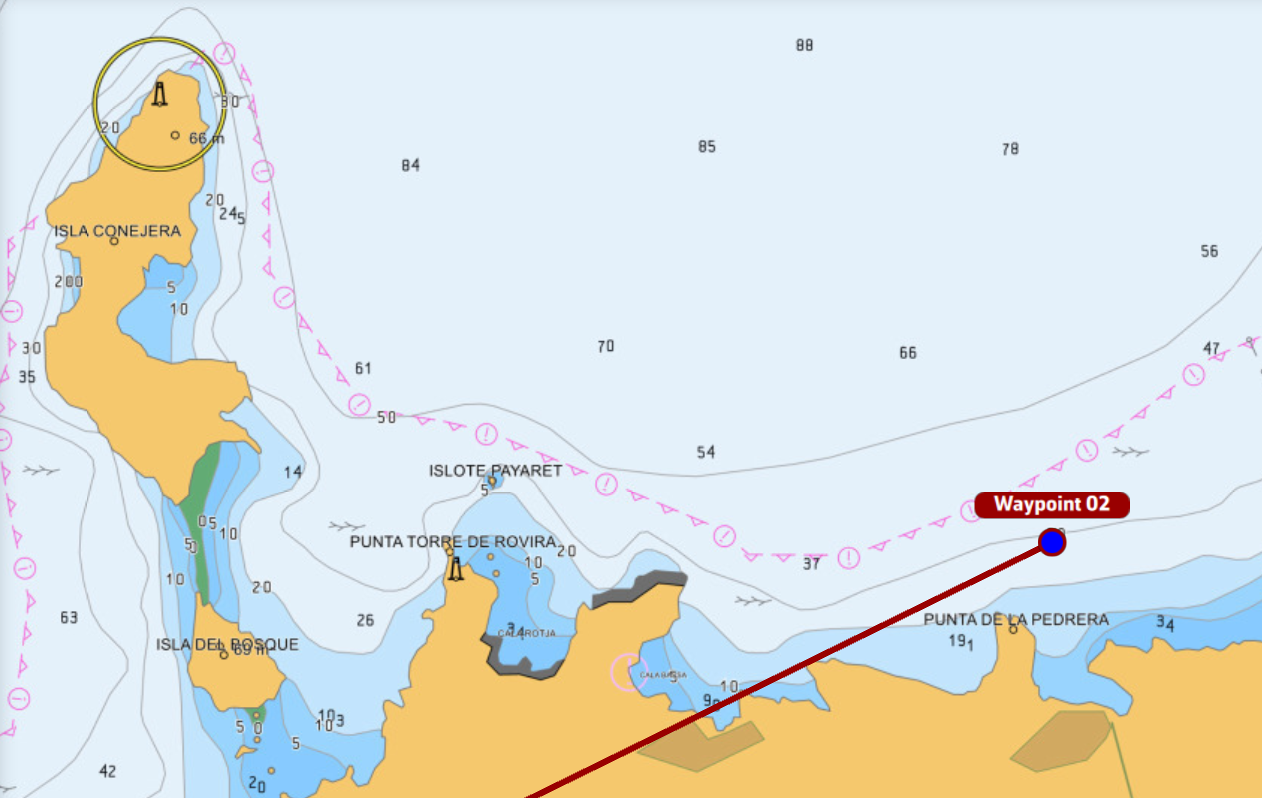
As illustrated, the route cuts directly across land, and the departure and arrival points are at sea — not in the harbours!

Wind GRIB

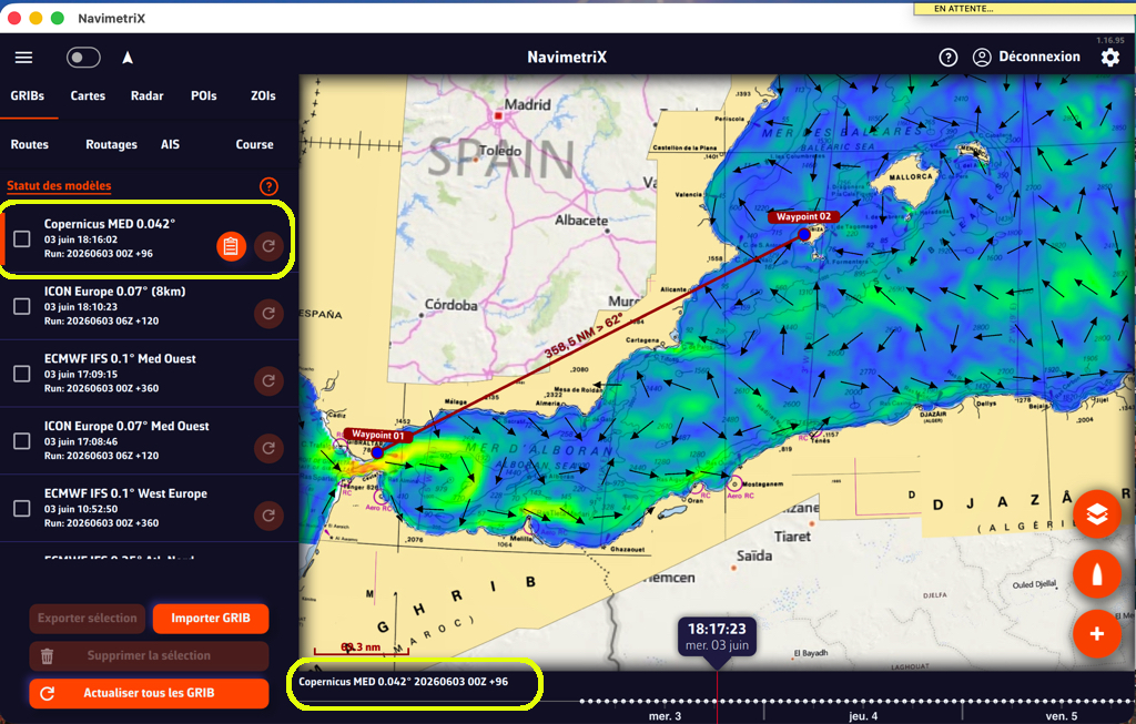
Current GRIB

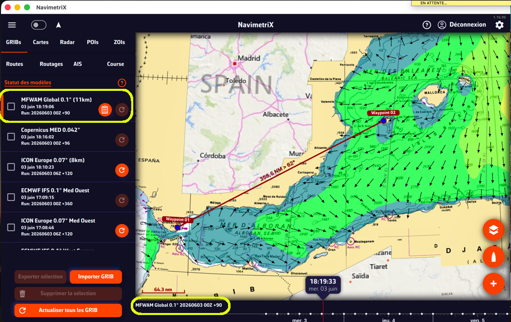
Wave GRIB

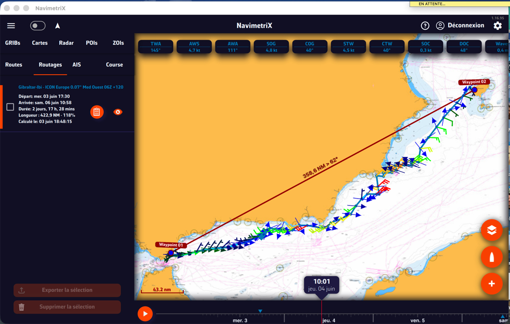
3. The Routing Calculation

The routing calculation is launched using the “PLUS” action button:

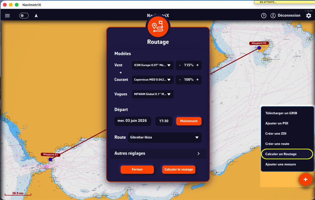
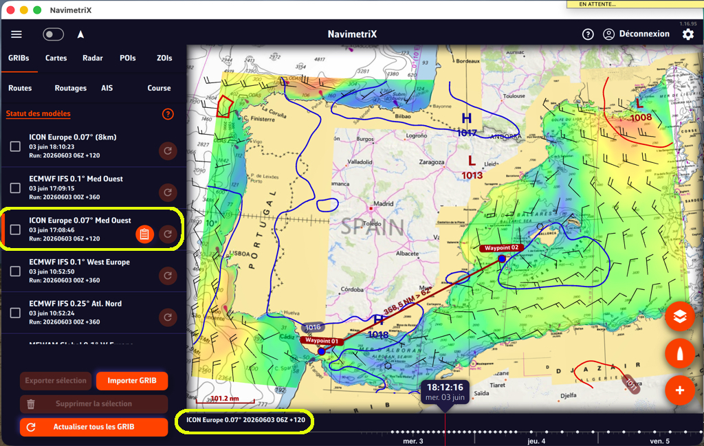
Select the GRIB files appropriate for the length of the route, with the highest resolution available for the geographic area in question.

In this example, for a passage of approximately 700 nautical miles taking around 60 hours according to the polar, the ICON Europe 0.07° (5NM) or IFS 0.1° (6NM) models are suitable for the Mediterranean basin.

The first routing, in conditions of highly variable wind and alternating currents in the Alboran Sea, produces a fairly tight coastal track. A closer look is needed.

Departure

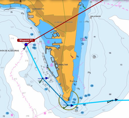
The departure correctly rounds the Point of Europe.

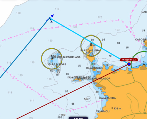
Arrival

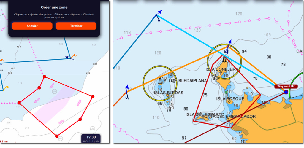
The arrival at Port des Torrent correctly rounds the islands off the coast, despite the very light wind.

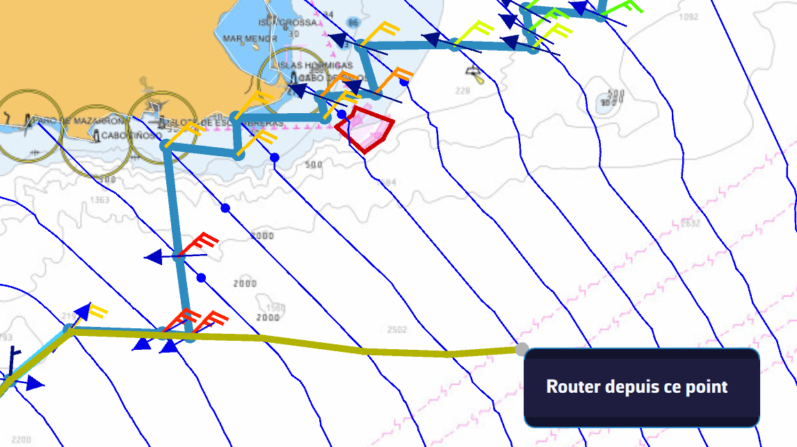
However, the passage south of Cabo de Palos involves tight tacks between the coast and the TSS. Passing further offshore may be preferable. We will use a “pivot point” to modify the routing in that area.

Select the routing in the left panel and display the isochrones in the “Display” layer. By dragging the chart under the yellow line that appears, you sweep through the isochrones to find a new point from which to “pivot” the routing. A right-click or press on the chosen point relaunches the routing from that pivot point.

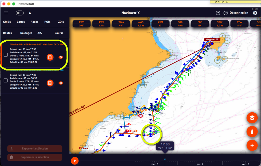
The routing resumes from the pivot point to the destination. You can compare the two routing results in the left panel, mainly the impact of the pivot point on the passage duration.

Be sure to create a ZOI for the TSS off Cabo de Palos, and also a ZOI at the destination to navigate around the surrounding islands.

4. Routing Settings

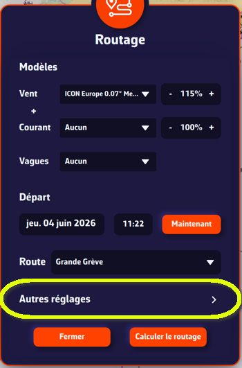
The preliminary routing settings should be configured according to your speed polar — activated in the “My Boat” settings — and your sailing style. They are described in detail in the FAQ and are persistent.

However, in certain cases you can modify them for a specific routing directly in the routing calculation window, without affecting your general settings.

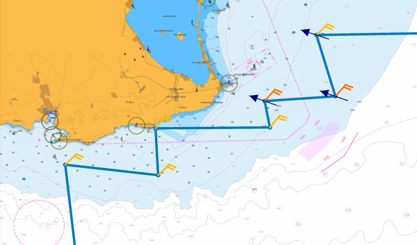
5. Special Case: Multi-GRIB Routing

You can choose several wind models for a passage. The aim is to select a wind model with sufficient temporal coverage for the entire route, and a higher-resolution model to refine the first part of the passage. The longer model takes over from the shorter one in time.

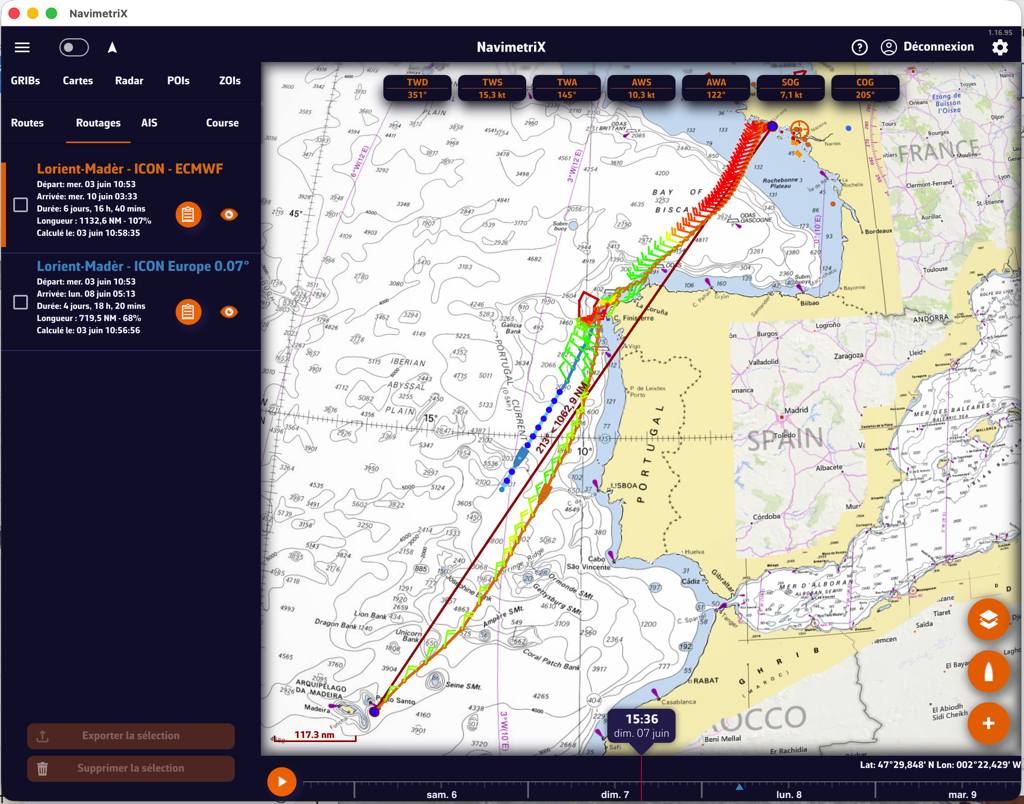
In the example above, a first Lorient–Madeira routing is calculated using an ICON Europe model at 5 days. At the end of the GRIB file it stops, resulting in a partial routing (in blue). A second routing is then performed by adding an IFS 0.1° model at 10 days. This one takes over from the first, ultimately providing greater precision (in orange).

Multi-GRIB routing implementation is detailed in the FAQ.

6. Recommendations

Polar adjustment: Polars are always optimistic (architect’s calculations). You will need to adjust their efficiency in different situations by observing your performance against the routings produced. You can decrease (most often) or increase efficiency “as you go.” In addition, the maximum TWS angle limits upwind and downwind have a significant impact on the relevance of routings at these boundary points of sail.

Isochrone interval setting: In the vast majority of cases, leave this on “Auto.” The calculation adapts the interval to the distance between two points, reducing it near departure and arrival. If you set a fixed interval, there is no point making it too short for passages longer than a few nautical miles — it adds no precision, demands significant computing power, and becomes counterproductive.

Constraint settings (max TWS, wave height): Be cautious with these constraints, as they risk producing impossible routings. Check the wind and wave forecasts along the route that you are likely to encounter. If the values are too high for your boat and crew, there is no point doing a routing: don’t leave! The colour-coded GRIB display — gradients or colour isobands — can help: as long as you are in the green, all is clear. As soon as it starts turning yellow, conditions are deteriorating; in red and magenta, stand down — unless you are a seasoned, experienced racer, of course!

Do not hesitate to consult the FAQ entries in the “Routing” category for more details.